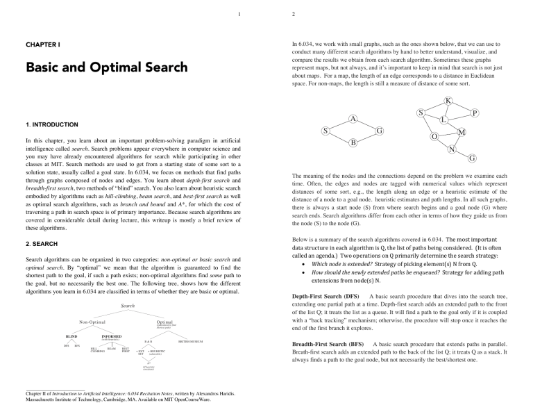
1 CHAPTER I Basic and Optimal Search 2 In 6.034, we work with small graphs, such as the ones shown below, that we can use to conduct many different search algorithms by hand to better understand, visualize, and compare the results we obtain from each search algorithm. Sometimes these graphs represent maps, but not always, and it’s important to keep in mind that search is not just about maps. For a map, the length of an edge corresponds to a distance in Euclidean space. For non-maps, the length is still a measure of distance of some sort. K 1. INTRODUCTION S In this chapter, you learn about an important problem-solving paradigm in artificial intelligence called search. Search problems appear everywhere in computer science and you may have already encountered algorithms for search while participating in other classes at MIT. Search methods are used to get from a starting state of some sort to a solution state, usually called a goal state. In 6.034, we focus on methods that find paths through graphs composed of nodes and edges. You learn about depth-first search and breadth-first search, two methods of “blind” search. You also learn about heuristic search embodied by algorithms such as hill-climbing, beam search, and best-first search as well as optimal search algorithms, such as branch and bound and A*, for which the cost of traversing a path in search space is of primary importance. Because search algorithms are covered in considerable detail during lecture, this writeup is mostly a brief review of these algorithms. 2. SEARCH Search algorithms can be organized in two categories: non-optimal or basic search and optimal search. By “optimal” we mean that the algorithm is guaranteed to find the shortest path to the goal, if such a path exists; non-optimal algorithms find some path to the goal, but no necessarily the best one. The following tree, shows how the different algorithms you learn in 6.034 are classified in terms of whether they are basic or optimal. Search Non-Optimal BLIND DFS S A Optimal (guaranteed to find shortest path) G B P L M O N G The meaning of the nodes and the connections depend on the problem we examine each time. Often, the edges and nodes are tagged with numerical values which represent distances of some sort, e.g., the length along an edge or a heuristic estimate of the distance of a node to a goal node. heuristic estimates and path lengths. In all such graphs, there is always a start node (S) from where search begins and a goal node (G) where search ends. Search algorithms differ from each other in terms of how they guide us from the node (S) to the node (G). Below is a summary of the search algorithms covered in 6.034. The most important data structure in each algorithm is Q, the list of paths being considered. (It is often called an agenda.) Two operations on Q primarily determine the search strategy: • Which node is extended? Strategy of picking element(s) N from Q. • How should the newly extended paths be enqueued? Strategy for adding path extensions from node(s) N. Depth-First Search (DFS) A basic search procedure that dives into the search tree, extending one partial path at a time. Depth-first search adds an extended path to the front of the list Q; it treats the list as a queue. It will find a path to the goal only if it is coupled with a “back tracking” mechanism; otherwise, the procedure will stop once it reaches the end of the first branch it explores. INFORMED (with heuristic) B&B BRITISH MUSEUM BFS HILL BEAM CLIMBING BEST FIRST + EXT. SET + HEURISTIC (admissible) A* (if heuristic consistent) Chapter II of Introduction to Artificial Intelligence: 6.034 Recitation Notes, written by Alexandros Haridis. Massachusetts Institute of Technology, Cambridge, MA. Available on MIT OpenCourseWare. Breadth-First Search (BFS) A basic search procedure that extends paths in parallel. Breath-first search adds an extended path to the back of the list Q; it treats Q as a stack. It always finds a path to the goal node, but not necessarily the best/shortest one. 3 Hill-climbing The basic depth-first search procedure turns into hill-climbing once we introduce heuristic quality measurements. In particular, we assume that there is a natural measure of distance from every node to the goal node and use that distance as a heuristic estimate of the remaining path to the goal. Note that hill-climbing sorts extended paths by their heuristic estimate before adding them to the front of the list Q. It is a variation of generate and test. 4 then the estimate added to the definitely known distance so far should be a good estimate of total path length. A* (A-star) A* has many variations but, traditionally, it is carried out with branch and bound augmented with an extended set and a consistent heuristic. Beam search The basic breadth-first search procedure turns into beam search when we sort the extended paths by their heuristic estimate and keep only a fixed number w of those partially extended paths while pruning the rest, i.e., we keep the best w paths in each level that we’ve extended in parallel, for a given number w. Best-first search Best-first search also uses a heuristic estimate to rank the partially extended paths. It is beam search with a w of 1. At each node, add partially extended paths to the list Q, sort the entire list by the partial paths’ heuristic estimates, and then extend the best of those paths. Where you add the partially extended paths to the list isn’t important, since the list will be sorted. Visualizing the list of partial paths British Museum Algorithm The British Museum algorithm relies on enumerating all possible paths in the search space and then choosing the best of those. In this sense, the British Museum algorithm is an instance of optimal search albeit an impractical one. In depth-first search we remove a partial path from the front of the list, extend the path to obtain one or more new partial paths, and we add those in the front of the list. We do the same in breadth-first search, only now we add the new partial paths at the back (bottom) of the list. Branch and Bound (B&B) In its simple form, branch and bound keeps track of all partial paths available and compares them in terms of what we call path length so far. (Note that path length is not the number of edges in the path, but rather the sum of distances along the edges in a path.) The shortest path in terms of length is extended one level, creating new partial paths. Next, these new paths are considered along with the remaining old ones. Again, the shortest path in terms of length is extended, and the process repeats until the goal node is reached. We have to extend all partial paths until they are as long as or longer than the complete path we’ve found, i.e., the one containing the goal node. This stopping condition guarantees that the path we’ve found is indeed the optimal/shortest one. B&B with an extended set This variation of the branch and bound procedure uses an extended set to keep track of the nodes we extend. Once we extend a partial path from a certain node, we add that node to the set. If we visit that node anew as we explore partial paths, we will not extend it again. B&B with a heuristic This variation of the branch and bound procedure uses a heuristic estimate of the remaining path length to the goal, in addition to the usual path length so far. The idea is that if the estimate about the remaining distance is admissible, We use a list to keep track of all the partial paths under consideration. The way in which it is populated, maintained, or sorted depends each time on the rules of the search algorithm. DFS Add in the front of the agenda as in a stack. BFS Add in the bottom of the agenda as in a queue. The following figure illustrates how the list behaves during beam search. After a whole level is extended following a breadth-first search strategy, we sort the entire list and keep the best w partial paths, for some given w (“beam width”).
