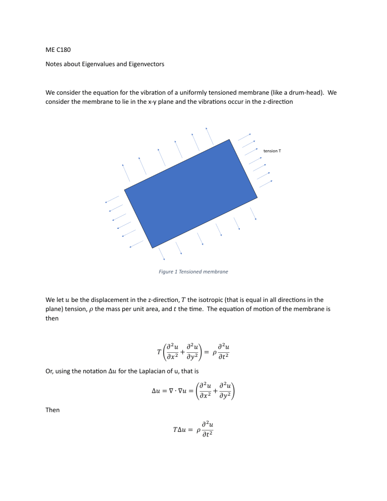
ME C180
Notes about Eigenvalues and Eigenvectors
We consider the equation for the vibration of a uniformly tensioned membrane (like a drum-head). We
consider the membrane to lie in the x-y plane and the vibrations occur in the z-direction
tension T
Figure 1 Tensioned membrane
We let 𝑢 be the displacement in the z-direction, 𝑇 the isotropic (that is equal in all directions in the
plane) tension, 𝜌 the mass per unit area, and 𝑡 the time. The equation of motion of the membrane is
then
𝑇(
𝜕2𝑢 𝜕2𝑢
𝜕2𝑢
+
=
𝜌
)
𝜕𝑥 2 𝜕𝑦 2
𝜕𝑡 2
Or, using the notation ∆𝑢 for the Laplacian of u, that is
∆𝑢 = ∇ ∙ ∇𝑢 = (
𝜕2𝑢 𝜕2𝑢
+
)
𝜕𝑥 2 𝜕𝑦 2
Then
𝑇∆𝑢 = 𝜌
𝜕2𝑢
𝜕𝑡 2
We can write the strong form of this equation then as
𝜌
𝜕2𝑢
− 𝑇∆𝑢 = 0
𝜕𝑡 2
We assume that the drumhead occupies a region Ω in the (x,y)-plane, and impose the condition that the
drum-head is fixed at the boundary of this region, 𝜕Ω, that is
𝑢 = 0 𝑜𝑛 𝜕Ω
Now we are interested at what frequencies the drumhead will vibrate, and what shapes those vibrations
will take. Hence we assume
𝑢 = Φ𝑒 −𝑖𝜔𝑡
Then
𝜕2𝑢
= −𝜔2 Φ𝑒 −𝑖𝜔𝑡
𝜕𝑡 2
So our equation is
−𝜔2 𝜌Φ − 𝑇∆Φ = 0
This is an example of the Helmholtz equation. Now we multiply by a test function 𝑤 and integrate:
∫ (−𝜔2 𝜌
Ω
𝜕2Φ
− 𝑇∆Φ) 𝑤 𝑑Ω = 0
𝜕𝑡 2
Now we integrate by parts on ∆Φ. So
∫ (−𝜔2 𝜌Φ𝑤 + 𝑇∇Φ ∙ ∇𝑤) 𝑑Ω = 0
Ω
Recognizing that both 𝜔 and Φ are unknowns, we use the standard shape functions to interpolate Φ and
𝑤, recognizing that that Φ = 𝑤 = 0 𝑜𝑛 𝜕Ω. Then
Φ = ∑ 𝑁𝐼 Φ𝐼
𝐼
w = ∑ 𝑁𝐼 w 𝐼
𝐼
So
w 𝐼 (−𝜔2 ∫ (𝜌𝑁𝐼 𝑁𝐽 ) 𝑑Ω + ∫ (𝑇∇𝑁𝐼 ∙ ∇𝑁𝐽 ) 𝑑Ω) Φ 𝐽 = 0
Ω
Ω
Let
𝑀𝐼𝐽 = ∫ (𝜌𝑁𝐼 𝑁𝐽 ) 𝑑Ω
Ω
𝐾𝐼𝐽 = ∫ (𝑇∇𝑁𝐼 ∙ ∇𝑁𝐽 ) 𝑑Ω
Ω
Defining the scalar 𝜆 via 𝜆 = 𝜔2 , then
∑(𝐾𝐼𝐽 − 𝜆𝑀𝐼𝐽 )Φ 𝐽 = 0 ∀ 𝐼
𝐽
This is an example of the discrete eigenvalue problem. This problem is characterized by the following:
1) The matrix [𝐾𝐼𝐽 ] is symmetric and positive semi-definite
2) The matrix [𝑀𝐼𝐽 ] is symmetric and positive definite
There DO NOT exist solutions to this equation for all values of 𝜆. The values of 𝜆 for which solutions do
exist are called “eigenvalues”. The eigenvalues are determined by the characteristic equation
det([𝐾] − 𝜆[𝑀]) = 0
IF the matrices [𝐾] and [𝑀] are size 𝑁 × 𝑁, then this equation is an 𝑁th-degree polynomial, with 𝑁
roots, all ≥ 0. If [𝐾] and [𝑀] are positive definite, then all the roots are all > 0. Some of the roots may
be repeated, so there may not be 𝑁 distinct eigenvalues, though practically speaking a numerical
algorithm will usually find 𝑁 distinct eigenvalues, with “repeated” eigenvalue simply having almost the
same value.
We usually list the eigenvalues 𝜆 which satisfy this equation from lowest to highest, so we speak of 𝜆𝐽 ,
the 𝐽th eigenvalue, and 𝜆1 the “lowest eigenvalue”. For each eigenvalue there is an associate vector
[Φ]𝐽 , which satisfies the equation
([𝐾] − 𝜆𝐽 [𝑀])[Φ]𝐽 = [0]
We call [Φ]𝐽 the eigenvector corresponding to eigenvalue 𝜆𝐽
We can construct eigenvalues and eigenvectors for general systems from solid mechanics and heat
transfer.
We remember that from heat transfer we construct a discrete system that looks like
[𝑀][𝑇̇] + [𝐾][𝑇] = [𝐹]
And we can write the discrete system for solid mechanics as
[𝑀][𝑢̈ ] + [𝐾][𝑢] = [𝐹]
For both cases, we are interested in the system for the homogeneous case, that is [𝐹] = 0.
For heat transfer, the eigenvalue system comes from assuming a solution of the form
[𝑇] = 𝑒 −𝜆𝑡 [Φ]
For solid mechanics, as in the vibrating drum-head example above, the system comes from assuming a
solution of the form
[𝑇] = 𝑒 −𝑖𝜔𝑡 [Φ]
With again
𝜆 = 𝜔2
Another term for eigenvalues is “modes” and the corresponding term for eigenvectors is “mode shapes”.
For solid mechanics, if a system is vibrating at or near the frequency 𝜔𝐽 corresponding to the eigenvalue
𝜆𝐽 then the vibrations take the “shape” of the mode[Φ]𝐽 , since
([𝐾] − 𝜆𝐽 [𝑀])[Φ]𝐽 = [0]
The “lowest mode” for a beam tends to be the beam bending in the softest direction, similar for a guitar
string the lowest mode corresponds to the lowest note the guitar string can play.
The classical software package which is used to determine modes and mode shapes is ARPACK
https://en.wikipedia.org/wiki/ARPACK
Another set of software packages but with more restricted usage are packages based upon the LOBPCG
method, of which there are numerous software package available:
https://en.wikipedia.org/wiki/LOBPCG
We note that there are N modes corresponding to the N degrees-of-freedom in a system, which of
course can be very many for a large finite-element mesh. But typically we are only interested in a few
modes – often those are the lowest or highest modes, or perhaps we may be interested in the modes
centered around a certain excitation frequency, for example the frequency of revolution of a helicopter
rotor. Fortunately both of these software packages can be configured to find modes centered around
either the lowest (e.g. close to zero) or highest mode, or even around another frequency. They are
iterative methods, so the more modes you ask for, the longer the algorithm takes.
We talk of the “lowest mode” and the “highest mode”, but what do those mean?
For heat transfer, the “highest mode” corresponds to the time it takes to “heat up” one node of the
problem – it is related to the largest stable time step. The “lowest mode” typically is related to the time
it takes to heat up the entire system. Both of these concepts were discussed further in the section of
notes about “Time Integration and the Wine Cellar Problem”.
For solid mechanics, the “highest mode” is the highest frequency of vibration – typically associated with
the vibration of a single node. Just like in thermal mechanics, this is related to the largest stable time
step. The “lowest mode” is the lowest frequency of vibration, think of the softest mode of beambending, or the lowest note a guitar string can play. Typically, engineers want to make sure the lowest
mode has a frequency higher than any anticipated excitation (forcing function). If a mode is “excited”
because a forcing function is at or near it’s natural frequency, the vibration amplitudes can become very
large.
It should be noted that an eigenvector is typically normalized. That is because, if [Φ]𝐽 satisfies
([𝐾] − 𝜆𝐽 [𝑀])[Φ]𝐽 = [0] , then so does 𝐶[Φ]𝐽 , for any scalar 𝐶.
The study of linear system vibrations using eigenvectors and eigenvalues is called “modal analysis”.
There is a rich literature in this field and many specialized software packages for analyzing mode shapes
and comparing to experiment.
Advanced topic not on the final but useful to know:
There are two common ways to normalize the eigenvectors. The first is simply normalizing
the magnitude to 1, that is
[Φ]𝑇𝐽 [Φ]𝐽 = 1
The second is “mass-normalization”
[Φ]𝑇𝐽 [𝑀][Φ]𝐽 = 1
Advanced topic not on the final, but useful to know:
If 𝜆𝐽 is a repeated eigenvalue, then there exists more than one eigenvector for that eigenvalue,
more particularly the eigenvectors for a repeated eigenvalue form a subspace of dimension M,
where M is the number of times the eigenvector is repeated. Practically-speaking this isn’t as
important because numerically one normally gets, rather than exactly repeated eigenvalues,
instead a number of eigenvalues which are very close to one another. However, it should be
noted in this case that the order is a numerical artifact, so small changes to the problem setup
may result in a different order, and entirely different eigenvectors, though still spanning the
same subspace.
Advanced topic not on the final, but useful to know:
If we mass-normalize the eigenvectors, then
[Φ]𝑇𝐽 [𝑀][Φ]𝐽 = 1
And
[Φ]𝑇𝐽 [𝑀][Φ]𝐽 = 𝜆𝐽
Since there are N eigenvectors, and one can show that they are linearly independent, that is one
can determine coefficients 𝑎𝐽 such that any vector [u] can be written as the sum of eigenvectors.
[u] = ∑ 𝑎𝐽 [Φ]𝐽
𝐽
In fact, it can be shown that, if we construct a square matrix [𝑄] with each column of [𝑄]
corresponding to an eigenvector we can construct a
[𝑄] = [[Φ]1
[Φ]2
… [Φ]𝑁 ]
Then
1
[𝑄]𝑇 [𝑀][𝑄] = [0
0
0
0
1
0
0
0
0
…
0
0
0
]
0
1
And
𝜆1
0
[𝑄]𝑇 [𝐾][𝑄] = [
0
0
0
𝜆2
0
0
0 0
0 0
]
… 0
0 𝜆𝑁
So in the expressed in “eigenvector space”, also known as “modal coordinates” the discrete
system looks like for thermal mechanics
𝑞̇ 𝐽 − 𝜆𝐽 𝑞𝐽 = 0
And for solid mechanics
𝑞̈ 𝐽 − 𝜆𝐽 𝑞𝐽 = 0
That is, after having transformed the system into modal coordinates, each “mode” has become
decoupled from every other mode, now we have 𝑁 independent ODE’s, instead of a system of
coupled ODE’s as before. We can transform back and forth via
[𝑢] = [𝑄][𝑞]
[𝑞] = [𝑄]𝑇 [𝑞]