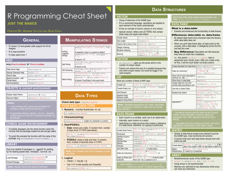
R Programming Cheat Sheet
just the basics
Created By: Arianne Colton and Sean Chen
General
• R version 3.0 and greater adds support for 64 bit
integers
• R is case sensitive
• R index starts from 1
Manipulating Strings
Putting
Together
Strings
HELP
help(functionName) or ?functionName
Split String
Help Home Page
help.start()
Get Substring
apropos('mea')
Match String
Special Character Help
Search Help
Search Function - with
Partial Name
See Example(s)
help('[')
help.search(..)or ??..
example(topic)
Objects in current environment
Display Object Name
Remove Object
objects() or ls()
rm(object1, object2,..)
paste('string1', 'string2', sep
= '/')
# separator ('sep') is a space by default
paste(c('1', '2'), collapse =
'/')
# returns '1/2'
stringr::str_split(string = v1,
pattern = '-')
# returns a list
stringr::str_sub(string = v1,
start = 1, end = 3)
isJohnFound <- stringr::str_
detect(string = df1$col1,
pattern = ignore.case('John'))
# returns True/False if John was found
df1[isJohnFound, c('col1',
...)]
Data Types
Notes:
Check data type: class(variable)
1. .name starting with a period are accessible but
invisible, so they will not be found by ‘ls’
1. Numeric - includes float/double, int, etc.
2. To guarantee memory removal, use ‘gc’, releasing
unused memory to the OS. R performs automatic ‘gc’
periodically
Symbol Name Environment
• If multiple packages use the same function name the
function that the package loaded the last will get called.
• To avoid this precede the function with the name of the
package. e.g. packageName::functionName(..)
Library
Only trust reliable R packages i.e., 'ggplot2' for plotting,
'sp' for dealing spatial data, 'reshape2', 'survival', etc.
Load Package
Unload Package
library(packageName)or
require(packageName)
detach(packageName)
Note: require() returns the status(True/False)
Four Basic Data Types
is.numeric(variable)
2. Character(string)
nchar(variable) # length of a character or numeric
3. Date/POSIXct
• Date: stores just a date. In numeric form, number
of days since 1/1/1970 (see below).
date1 <- as.Date('2012-06-28'),
as.numeric(date1)
• POSIXct: stores a date and time. In numeric
form, number of seconds since 1/1/1970.
date2 <- as.POSIXct('2012-06-28 18:00')
Note: Use 'lubridate' and 'chron' packages to work
with Dates
4. Logical
• (TRUE = 1, FALSE = 0)
• Use ==/!= to test equality and inequality
as.numeric(TRUE) => 1
Data Structures
Vector
• Group of elements of the SAME type
• R is a vectorized language, operations are applied to
each element of the vector automatically
• R has no concept of column vectors or row vectors
• Special vectors: letters and LETTERS, that contain
lower-case and upper-case letters
Create Vector
v1 <- c(1, 2, 3)
Get Length
length(v1)
Check if All or Any is True all(v1); any(v1)
Integer Indexing
v1[1:3]; v1[c(1,6)]
Boolean Indexing
v1[is.na(v1)] <- 0
c(first = 'a', ..)or
names(v1) <- c('first', ..)
Naming
Factor
• as.factor(v1) gets you the levels which is the
number of unique values
• Factors can reduce the size of a variable because they
only store unique values, but could be buggy if not
used properly
list
Store any number of items of ANY type
Create List
Create Empty List
list1 <- list(first = 'a', ...)
vector(mode = 'list', length
= 3)
Get Element
list1[[1]] or list1[['first']]
Append Using
list1[[6]] <- 2
Numeric Index
Append Using Name list1[['newElement']] <- 2
Note: repeatedly appending to list, vector, data.frame
etc. is expensive, it is best to create a list of a certain
size, then fill it.
data.frame while using single-square brackets, use
‘drop’: df1[, 'col1', drop = FALSE]
data.table
What is a data.table
• Extends and enhances the functionality of data.frames
Differences: data.table vs. data.frame
• By default data.frame turns character data into factors,
while data.table does not
• When you print data.frame data, all data prints to the
console, with a data.table, it intelligently prints the first
and last five rows
• Key Difference: Data.tables are fast because
they have an index like a database.
i.e., this search, dt1$col1 > number, does a
sequential scan (vector scan). After you create a key
for this, it will be much faster via binary search.
Create data.table from data.frame data.table(df1)
dt1[, 'col1', with
= FALSE] or
Index by Column(s)*
dt1[, list(col1)]
Show info for each data.table in tables()
memory (i.e., size, ...)
key(dt1)
Show Keys in data.table
Create index for col1 and
setkey(dt1, col1)
reorder data according to col1
dt1[c('col1Value1',
Use Key to Select Data
'col1Value2'), ]
dt1[J('1', c('2', '3')), ]
Multiple Key Select
dt1[, list(col1 =
mean(col1)), by =
col2]
**
Aggregation
dt1[, list(col1 =
mean(col1), col2Sum
= sum(col2)), by =
list(col3, col4)]
* Accessing columns must be done via list of actual
names, not as characters. If column names are
characters, then "with" argument should be set to
FALSE.
data.frame
• Each column is a variable, each row is an observation
• Internally, each column is a vector
• idata.frame is a data structure that creates a reference
to a data.frame, therefore, no copying is performed
df1 <- data.frame(col1 = v1,
Create Data Frame col2 = v2, v3)
nrow(df1); ncol(df1); dim(df1)
Dimension
Get/Set Column
names(df1)
Names
names(df1) <- c(...)
Get/Set Row
rownames(df1)
Names
rownames(df1) <- c(...)
head(df1, n = 10); tail(...)
Preview
Get Data Type
class(df1) # is data.frame
df1['col1']or df1[1];†
Index by Column(s) df1[c('col1', 'col3')] or
df1[c(1, 3)]
Index by Rows and df1[c(1, 3), 2:3] # returns data
Columns
from row 1 & 3, columns 2 to 3
† Index method: df1$col1 or df1[, 'col1'] or
df1[, 1] returns as a vector. To return single column
** Aggregate and d*ply functions will work, but built-in
aggregation functionality of data table is faster
Matrix
• Similar to data.frame except every element must be
the SAME type, most commonly all numerics
• Functions that work with data.frame should work with
matrix as well
Create Matrix matrix1 <- matrix(1:10, nrow = 5), # fills
rows 1 to 5, column 1 with 1:5, and column 2 with 6:10
Matrix
matrix1 %*% t(matrix2)
Multiplication # where t() is transpose
Array
•
•
•
•
Multidimensional vector of the SAME type
array1 <- array(1:12, dim = c(2, 3, 2))
Using arrays is not recommended
Matrices are restricted to two dimensions while array
can have any dimension
Data Munging
Apply (apply, tapply, lapply, mapply)
• Apply - most restrictive. Must be used on a matrix, all
elements must be the same type
• If used on some other object, such as a data.frame, it
will be converted to a matrix first
apply(matrix1, 1 - rows or 2 - columns,
function to apply)
# if rows, then pass each row as input to the function
• By default, computation on NA (missing data) always
returns NA, so if a matrix contains NAs, you can
ignore them (use na.rm = TRUE in the apply(..)
which doesn’t pass NAs to your function)
lapply
Applies a function to each element of a list and returns
the results as a list
sapply
Same as lapply except return the results as a vector
Note: lapply & sapply can both take a vector as input, a
vector is technically a form of list
Aggregate (SQL groupby)
• aggregate(formulas, data, function)
• Formulas: y ~ x, y represents a variable that we
want to make a calculation on, x represents one or
more variables we want to group the calculation by
• Can only use one function in aggregate(). To apply
more than one function, use the plyr() package
In the example below diamonds is a data.frame; price,
cut, color etc. are columns of diamonds.
aggregate(price ~ cut, diamonds, mean)
# get the average price of different cuts for the diamonds
aggregate(price ~ cut + color, diamonds,
mean) # group by cut and color
aggregate(cbind(price, carat) ~ cut,
diamonds, mean) # get the average price and average
carat of different cuts
Plyr ('split-apply-combine')
• ddply(), llply(), ldply(), etc. (1st letter = the type of
input, 2nd = the type of output
• plyr can be slow, most of the functionality in plyr
can be accomplished using base function or other
packages, but plyr is easier to use
ddply
Takes a data.frame, splits it according to some
variable(s), performs a desired action on it and returns a
data.frame
llply
• Can use this instead of lapply
• For sapply, can use laply (‘a’ is array/vector/matrix),
however, laply result does not include the names.
DPLYR (for data.frame ONLY)
• Basic functions: filter(), slice(), arrange(), select(),
rename(), distinct(), mutate(), summarise(),
Functions and Controls
group_by(), sample_n()
• Chain functions
df1 %>% group_by(year, month) %>%
select(col1, col2) %>% summarise(col1mean
= mean(col1))
• Much faster than plyr, with four types of easy-to-use
joins (inner, left, semi, anti)
• Abstracts the way data is stored so you can work with
data frames, data tables, and remote databases with
the same set of functions
Helper functions
each() - supply multiple functions to a function like aggregate
aggregate(price ~ cut, diamonds, each(mean,
median))
Data
Load Data from CSV
• Read csv
read.table(file = url or filepath, header =
TRUE, sep = ',')
• “stringAsFactors” argument defaults to TRUE, set it to
FALSE to prevent converting columns to factors. This
saves computation time and maintains character data
• Other useful arguments are "quote" and "colClasses",
specifying the character used for enclosing cells and
the data type for each column.
• If cell separator has been used inside a cell, then use
read.csv2() or read delim2() instead of read.
table()
Database
Connect to
Database
Query
Database
Close
Connection
db1 <- RODBC::odbcConnect('conStr')
df1 <- RODBC::sqlQuery(db1, 'SELECT
..', stringAsFactors = FALSE)
RODBC::odbcClose(db1)
• Only one connection may be open at a time. The
connection automatically closes if R closes or another
connection is opened.
• If table name has space, use [ ] to surround the table
name in the SQL string.
• which() in R is similar to ‘where’ in SQL
Included Data
R and some packages come with data included.
List Available Datasets
List Available Datasets in
a Specific Package
data()
data(package =
'ggplot2')
Missing Data (NA and NULL)
NULL is not missing, it’s nothingness. NULL is atomical
and cannot exist within a vector. If used inside a vector, it
simply disappears.
Check Missing Data
Avoid Using
is.na()
is.null()
Rearrange
say_hello <- function(first,
Create Function last = 'hola') { }
say_hello(first = 'hello')
Call Function
• R automatically returns the value of the last line of
code in a function. This is bad practice. Use return()
explicitly instead.
• do.call() - specify the name of a function either as
string (i.e. 'mean') or as object (i.e. mean) and provide
arguments as a list.
do.call(mean, args = list(first = '1st'))
if /else /else if /switch
Works with Vectorized Argument
Most Efficient for Non-Vectorized Argument
Works with NA *
Use &&, || **†
Use &, | ***†
Data Reshaping
if { } else
No
ifelse
Yes
Yes
No
No
Yes
Yes
No
No
Yes
* NA == 1 result is NA, thus if won’t work, it’ll be an
error. For ifelse, NA will return instead
** &&, || is best used in if, since it only compares the
first element of vector from each side
*** &, | is necessary for ifelse, as it compares every
element of vector from each side
† &&, || are similar to if in that they don’t work with
vectors, where ifelse, &, | work with vectors
• Similar to C++/Java, for &, |, both sides of operator
are always checked. For &&, ||, if left side fails, no
need to check the right side.
• } else, else must be on the same line as }
Graphics
reshape2.melt(df1, id.vars =
Melt Data - from c('col1', 'col2'), variable.
column to row name = 'newCol1', value.name =
'newCol2')
reshape2.dcast(df1, col1 +
Cast Data - from col2 ~ newCol1, value.var =
row to column 'newCol2')
If df1 has 3 more columns, col3 to col5, 'melting' creates
a new df that has 3 rows for each combination of col1
and col2, with the values coming from the respective col3
to col5.
Combine (mutiple sets into one)
1. cbind - bind by columns
data.frame from two vectors
cbind(v1, v2)
data.frame combining df1 and
df2 columns
cbind(df1, df2)
2. rbind - similar to cbind but for rows, you can assign
new column names to vectors in cbind
cbind(col1 = v1, ...)
3. Joins - (merge, join, data.table) using common keys
3.1 Merge
• by.x and by.y specify the key columns use in the
join() operation
• Merge can be much slower than the alternatives
merge(x = df1, y = df2, by.x = c('col1',
'col3'), by.y = c('col3', 'col6'))
3.2 Join
• Join in plyr() package works similar to merge but
much faster, drawback is key columns in each
table must have the same name
• join() has an argument for specifying left, right,
inner joins
join(x = df1, y = df2, by = c('col1',
'col3'))
Default basic graphic
3.3 data.table
hist(df1$col1, main = 'title', xlab = 'x
axis label')
dt1 <- data.table(df1, key = c('1',
'2')), dt2 <- ...‡
plot(col2 ~ col1, data = df1),
aka y ~ x or plot(x, y)
lattice and ggplot2 (more popular)
• Initialize the object and add layers (points, lines,
histograms) using +, map variable in the data to an
axis or aesthetic using ‘aes’
ggplot(data = df1) + geom_histogram(aes(x
= col1))
• Normalized histogram (pdf, not relative frequency
histogram)
ggplot(data = df1) + geom_density(aes(x =
col1), fill = 'grey50')
• Left Join
dt1[dt2]
‡ Data table join requires specifying the keys for the data
tables
Created by Arianne Colton and Sean Chen
data.scientist.info@gmail.com
Based on content from
'R for Everyone' by Jared Lander
Updated: December 2, 2015