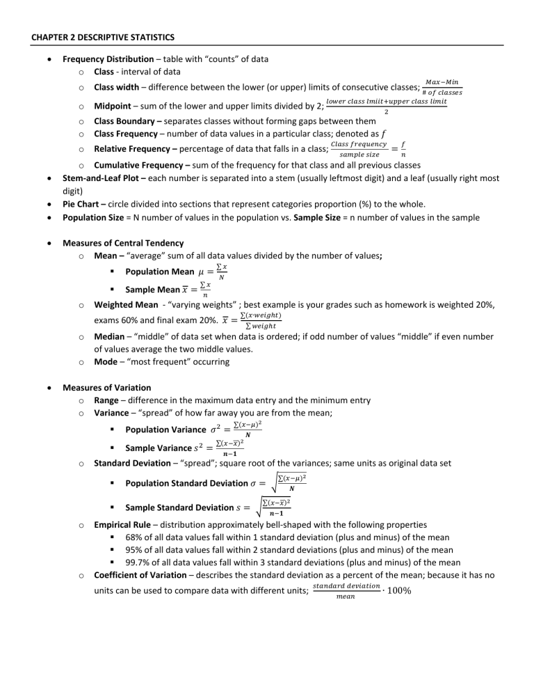
CHAPTER 2 DESCRIPTIVE STATISTICS
•
Frequency Distribution – table with “counts” of data
o Class - interval of data
o
Class width – difference between the lower (or upper) limits of consecutive classes;
o
Midpoint – sum of the lower and upper limits divided by 2;
o
Relative Frequency – percentage of data that falls in a class;
o
o
•
•
•
•
2
Class Boundary – separates classes without forming gaps between them
Class Frequency – number of data values in a particular class; denoted as 𝑓𝑓
𝐶𝐶𝐶𝐶𝐶𝐶𝐶𝐶𝐶𝐶 𝑓𝑓𝑓𝑓𝑓𝑓𝑓𝑓𝑓𝑓𝑓𝑓𝑓𝑓𝑓𝑓𝑓𝑓
𝑠𝑠𝑠𝑠𝑠𝑠𝑠𝑠𝑠𝑠𝑠𝑠 𝑠𝑠𝑠𝑠𝑠𝑠𝑠𝑠
=
𝑓𝑓
𝑛𝑛
o Cumulative Frequency – sum of the frequency for that class and all previous classes
Stem-and-Leaf Plot – each number is separated into a stem (usually leftmost digit) and a leaf (usually right most
digit)
Pie Chart – circle divided into sections that represent categories proportion (%) to the whole.
Population Size = N number of values in the population vs. Sample Size = n number of values in the sample
Measures of Central Tendency
o Mean – “average” sum of all data values divided by the number of values;


o
o
o
•
𝑀𝑀𝑀𝑀𝑀𝑀−𝑀𝑀𝑀𝑀𝑀𝑀
# 𝑜𝑜𝑜𝑜 𝑐𝑐𝑐𝑐𝑐𝑐𝑐𝑐𝑐𝑐𝑐𝑐𝑐𝑐
𝑙𝑙𝑙𝑙𝑙𝑙𝑙𝑙𝑙𝑙 𝑐𝑐𝑐𝑐𝑐𝑐𝑐𝑐𝑐𝑐 𝑙𝑙𝑙𝑙𝑙𝑙𝑙𝑙𝑙𝑙+𝑢𝑢𝑢𝑢𝑢𝑢𝑢𝑢𝑢𝑢 𝑐𝑐𝑐𝑐𝑐𝑐𝑐𝑐𝑐𝑐 𝑙𝑙𝑙𝑙𝑙𝑙𝑙𝑙𝑙𝑙
Population Mean 𝜇𝜇 =
Sample Mean 𝑥𝑥 =
∑ 𝑥𝑥
𝑛𝑛
∑ 𝑥𝑥
𝑁𝑁
Weighted Mean - “varying weights” ; best example is your grades such as homework is weighted 20%,
exams 60% and final exam 20%. 𝑥𝑥 =
∑(𝑥𝑥∙𝑤𝑤𝑤𝑤𝑤𝑤𝑤𝑤ℎ𝑡𝑡)
∑ 𝑤𝑤𝑤𝑤𝑤𝑤𝑤𝑤ℎ𝑡𝑡
Median – “middle” of data set when data is ordered; if odd number of values “middle” if even number
of values average the two middle values.
Mode – “most frequent” occurring
Measures of Variation
o Range – difference in the maximum data entry and the minimum entry
o Variance – “spread” of how far away you are from the mean;


o

o
2
Sample Variance 𝑠𝑠 =
∑(𝑥𝑥−𝜇𝜇)2
∑(𝑥𝑥−𝑥𝑥)2
𝒏𝒏−𝟏𝟏
𝑵𝑵
Standard Deviation – “spread”; square root of the variances; same units as original data set

o
Population Variance 𝜎𝜎 2 =
Population Standard Deviation 𝜎𝜎 = �
Sample Standard Deviation 𝑠𝑠 = �
∑(𝑥𝑥−𝜇𝜇)2
𝑵𝑵
∑(𝑥𝑥−𝑥𝑥)2
𝒏𝒏−𝟏𝟏
Empirical Rule – distribution approximately bell-shaped with the following properties
 68% of all data values fall within 1 standard deviation (plus and minus) of the mean
 95% of all data values fall within 2 standard deviations (plus and minus) of the mean
 99.7% of all data values fall within 3 standard deviations (plus and minus) of the mean
Coefficient of Variation – describes the standard deviation as a percent of the mean; because it has no
units can be used to compare data with different units;
𝑠𝑠𝑠𝑠𝑠𝑠𝑠𝑠𝑠𝑠𝑠𝑠𝑠𝑠𝑠𝑠 𝑑𝑑𝑑𝑑𝑑𝑑𝑑𝑑𝑑𝑑𝑑𝑑𝑑𝑑𝑑𝑑𝑑𝑑
𝑚𝑚𝑚𝑚𝑚𝑚𝑚𝑚
∙ 100%
•
Measures of Position
o Quartiles – divide ordered data in equal parts; Q1 25%; Q2 50% (median); Q3 75%; Q4 100%
o Interquartile range (IQR) - difference between the third and first quartiles; Q3 – Q1
o Five Number Summary - used for constructing a boxplot
 Minimum Value
 Q1
 Q2 (median)
 Q3
 Maximum Value