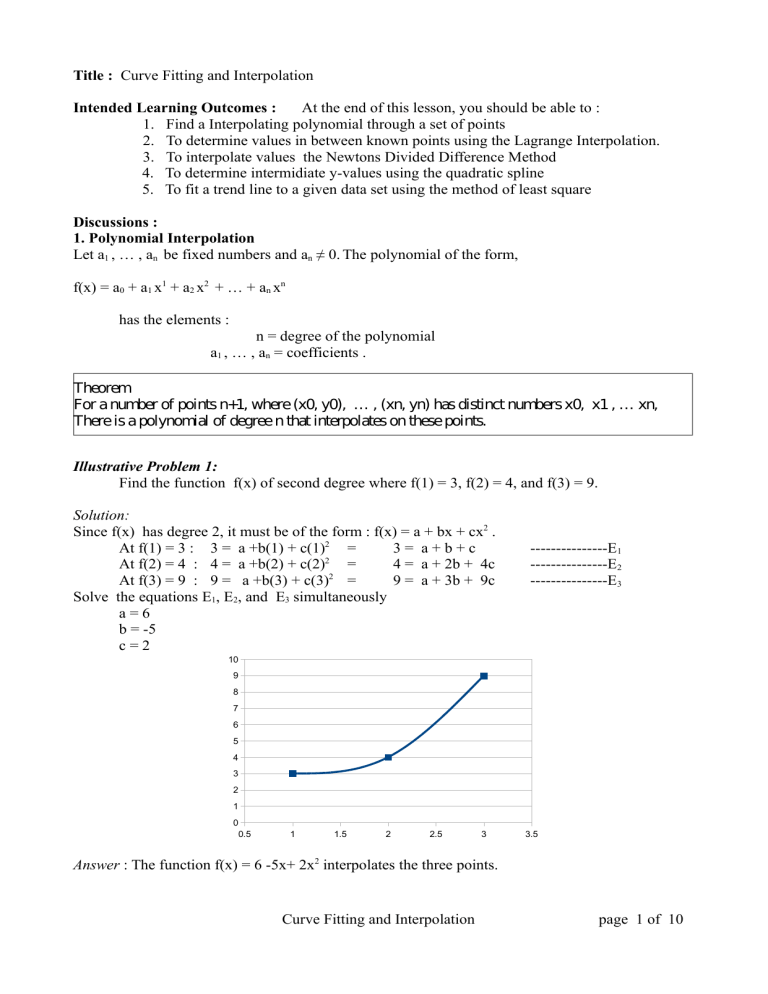
Title : Curve Fitting and Interpolation
Intended Learning Outcomes :
At the end of this lesson, you should be able to :
1. Find a Interpolating polynomial through a set of points
2. To determine values in between known points using the Lagrange Interpolation.
3. To interpolate values the Newtons Divided Difference Method
4. To determine intermidiate y-values using the quadratic spline
5. To fit a trend line to a given data set using the method of least square
Discussions :
1. Polynomial Interpolation
Let a1 , … , an be fixed numbers and an ≠ 0. The polynomial of the form,
f(x) = a0 + a1 x1 + a2 x2 + … + an xn
has the elements :
n = degree of the polynomial
a1 , … , an = coefficients .
Theorem
For a number of points n+1, where (x0, y0), … , (xn, yn) has distinct numbers x0, x1 , … xn,
There is a polynomial of degree n that interpolates on these points.
Illustrative Problem 1:
Find the function f(x) of second degree where f(1) = 3, f(2) = 4, and f(3) = 9.
Solution:
Since f(x) has degree 2, it must be of the form : f(x) = a + bx + cx2 .
At f(1) = 3 : 3 = a +b(1) + c(1)2 =
3= a+b+c
At f(2) = 4 : 4 = a +b(2) + c(2)2 =
4 = a + 2b + 4c
At f(3) = 9 : 9 = a +b(3) + c(3)2 =
9 = a + 3b + 9c
Solve the equations E1, E2, and E3 simultaneously
a=6
b = -5
c=2
---------------E1
---------------E2
---------------E3
10
9
8
7
6
5
4
3
2
1
0
0.5
1
1.5
2
2.5
3
3.5
Answer : The function f(x) = 6 -5x+ 2x2 interpolates the three points.
Curve Fitting and Interpolation
page 1 of 10
2. Lagrange Interpolation
Usage : To determine values in between known points in a data set
Lagrange interpolating polynomial can be written as
n
f n ( x )= Σ Li ( x ) f ( x i )
i= 0
n
Π x−x j
where : Li ( x )=
Π → defined as "product of"
j= 0 x i −x j
j≠i
For Example
1st degree :
x−x 1
x−x 0
f 1 ( x )=
f ( x o)+
f ( x 1)
x 0 −x 1
x1 −x 0
2nd degree :
f 3 ( x )=
f 2 ( x )=
3nd degree :
( x−x 1 )( x−x 2 )( x−x 3 )
( x 0 −x 1)( x 0 −x2 )( x 0 −x 3 )
f ( x o )+
( x−x 1 )( x−x 2 )
( x−x 0)( x−x 2 )
( x−x 0 )( x−x 1 )
f ( x o )+
f ( x 1 )+
f (x )
( x 0 −x 1 )( x 0 −x2 )
( x 1 −x 0)( x 1−x 2 )
( x 2−x 0 )( x 2 −x 1 ) 2
( x−x 0 )( x−x 2 )( x−x 3 )
( x−x 0)( x−x 1)( x−x 3)
( x−x 0 )( x−x 1 )( x−x 2 )
f ( x 1 )+
f ( x 2 )+
f ( x 3)
( x 1−x0 )( x1−x 2)( x 1−x 3)
( x 2−x 0 )( x 2 −x 1 )( x2−x 3 )
( x3−x 0)( x 3 −x 1 )( x3 −x 2 )
Illustrative Problem 2:
Using the data points shown below estimate the value of y if x = 1.6,
Use the Lagrange third - degree interpolation.
f 3 ( x )=
x
y = f(x)
x0 = 1
3
x1 = 2
4
x2 = 3
9
x3 = 4.6
18
Solution :
( x−x 1 )( x−x 2 )( x−x 3 )
( x 0 −x 1)( x 0 −x2 )( x 0 −x 3 )
f 3 ( 1 .6 )=
f ( x o )+
( x−x 0 )( x−x 2 )( x−x 3 )
( x−x 0)( x−x 1)( x−x 3)
( x−x 0 )( x−x 1 )( x−x 2 )
f ( x 1 )+
f ( x 2 )+
f ( x 3)
( x 1−x0 )( x1−x 2)( x 1−x 3)
( x 2−x 0 )( x 2 −x 1 )( x2−x 3 )
( x3−x 0)( x 3 −x 1 )( x3 −x 2 )
( 1. 6−2 )( 1. 6−3 )( 1. 6−4 . 6 ) (1 . 6−1 )( 1 .6−3 )( 1. 6−4 . 6 ) (1 . 6−1 )( 1 .6−2 )( 1. 6−4 . 6 ) (1 . 6−1 )( 1 .6−2 )( 1. 6−3 )
3+
4+
9+
18
(1−2 )(1−3 )( 1−4 .6 )
( 2−1 )( 2−3 )( 2−4 . 6 )
(3−1 )( 3−2 )( 3−4 . 6 )
( 4 . 6−1 )( 4 . 6−2 )( 4 . 6−3 )
f3(1.6) = 0.7 + 3.87692 – 2.025+0.40385 ≈ 2.9558
(answer)
Curve Fitting and Interpolation
page 2 of 10
3. Newton Divided Difference Method
Usage : To determine values in between known points in a data set
Newton Divided Difference interpolating polynomial can be written as
f n ( x ) =b o +b1 ( x−x o ) +b 2 ( x−x o )( x−x 1 ) + .. .b n ( x−x o )( x−x 1 ) . .. ( x−x n−1 )
where
b o =f ( x o )
b1 =f ( x1 ,xo )
.
.
.
bn =f ( x n ,x n−1 , . .. ,x 1 ,x0 )
the fuctions f are defined by
1st term
f ( x i ,x j ) =
f ( x j )−f ( x i )
nd
2 term
f ( x i ,x j ,x k )=
x j −xi
f ( x k ,x j ) −f ( x j ,xi )
x k −x i
.
.
.
nth term
f ( x n ,x n−1 ,. .. ,x 1 ,x 0 )=
f ( x n ,x n−1 ,. .. x 1 )−f ( x n−1 ,x n−2 ,. .. x 0 )
x n −x o
Illustrative Problem 2:
Using the data points shown below estimate the value of y if x = 1.6,
Use the Newton Divided Difference interpolation.
x
y = f(x)
x0 = 1
3
x1 = 2
4
x2 = 3
9
x3 = 4.6
18
Curve Fitting and Interpolation
page 3 of 10
Solution :
1. Prepare the table
i
x
f(x)
0
1
3
1
2
4
2
3
9
3
4.6
18
f(xi, xj)
f(xi, xj, xk)
f(xi, xj, xk, xl)
2. Extract the coefficients
b0 = 3
b1 = 1
b2 = 2
b3 = -0.488782
3. Use the formula to interpolate f(1.6)
f 3 ( x ) =bo +b1 ( x−x o ) +b 2 ( x−x o )( x−x 1 ) +b 3 ( x−x o )( x−x 1 )( x−x 2 )
f3(1.6) = 3+ 1(1.6-1) + 2(1.6-1)(1.6-2) -0.488782(1.6-1)(1.6-2)(1.6-3) ≈ 2.9558
interestingly
f2(1.6) = 3+ 1(1.6-1) + 2(1.6-1)(1.6-2)
f1(1.6) = 3+ 1(1.6-1)
(answer)
= 3.12 , quadratic
= 3.6 , linear
4. Quadratic Spline
Usage : To determine values in between known points in a data set using a spline
Consider the data set shown below. We want to draw a series of quadratic curve to link the
points given such that the overall curve is "smooth". There will be three quadratic functions for this
data set. One for each set of adjacent points.
20
x
1
3
6
10
y
1
-2
15
9
20
15
15
10
10
5
5
0
0
-5
0
2
4
6
8
10
12
Plotted points
-5 0
2
4
6
8
10
Smooth spline curve
The following conditions apply :
1. y-values at interior points must be equal
2. function values at end points are equal to y-values at end points
3. the slopes of the functions meeting at an interior point are equal
4. the second derivative at the first point is zero
Curve Fitting and Interpolation
page 4 of 10
12
Illustrative Problem 3: Consider the data set shown below. Obtain the quadratic spline to fit the
data set shown below. Estimate the value of y when x = 8.
x
1
3
6
10
y
1
-2
15
9
*Cubic Spline sample
Solution :
1. The are three quadratic functions to fit the data set
y1 = a1x2+ b1x +c1
y2 = a2x2+ b2x +c2
y3 = a3x2+ b3x +c3
2. Apply conditions
2.1 "y-values at interior points must be equal"
At x = 3;
a1(9) + b1(3) +c1 = -2
At x = 3;
a2(9) + b2(3) +c2 = -2
At x = 6;
At x = 6;
a2(36) + b2(6) +c2 = 15
a3(36) + b3(6) +c3 = 15
2.2 "function values at end points are equal to y-values at end points"
At x = 1;
a1(1) + b1(1) +c1 = 1
At x = 10;
a3(100) + b3(10) +c3= 9
2.3 "the slopes of the functions meeting at an interior point are equal"
y1' = y2'
At x = 3;
2a1(3) + b1 = 2a2(3) + b2
6a1 + b1 - 6a2 – b2 = 0
y2' = y3'
At x = 6;
2a2(6) + b2 = 2a3(6) + b3
12a2 + b2 - 12a3 – b3 = 0
2.4 "the second derivative at the first point is zero"
a1 = 0 , straight line from point1 to point 2
Curve Fitting and Interpolation
page 5 of 10
3. Determine the unknown constants
In matrix form
Solve the system of linear equations :
a1 = 0
b1= -0.8571
c 1= 1.8571
a2 = 2.1746
b2= -13.9048
c2= 20.1429
a3 = -3.4226
b3= 53.2619
c 3= -181.3571
4. Estimate the value of y when x = 8.
y3 = a3x2+ b3x +c3 = -3.4226(8)2 + 53.2619(8) -181.3571
, estimated value,
Answer.
5. Least Square Method
Linear Regression uses a straight line to fit a given set paired data set (x, y).
General Form
y = a + bx + e
where :
a = intercept
b = slope
e = error
we can express the equation in the form
e = y - a - bx
Minimize the error e using
S r =∑ e 2 =∑ ( y−a−bx )2
where :
n ∑ xy−∑ x ∑ y
b=
2
n ∑ x 2 − (∑ x )
a= ȳ−b x̄
Error Analysis
St = Σ(y- y)2
Curve Fitting and Interpolation
page 6 of 10
r 2=
S t −S r
St
,
-1 < r < 1.0 (perfect positive fit) correlation coefficient
Illustrative Problem 4: Fit a straight trend line using the method of least square from the following
data set, and find the trend values. Estimate y when x = 8. Determine the correlation coefficient r.
x
1
3
6
10
y
1
-2
15
9
Solution:
1. Populate the table
Σ
x
1
3
6
10
20
y
1
-2
15
9
23
x2
1
9
36
100
146
y2
1
4
225
81
311
xy
1
-6
90
90
175
2. Calculate the mean values , a, and b
∑ x = 20/ 4 = 5
x̄=
n
∑ y = 23 /4 = 5.75
ȳ=
n
b=
n ∑ xy−∑ x ∑ y
n ∑ x 2 − (∑ x )
b = 1.304348
2
=
4 ( 175 )−20 ( 23 )
2
4 (146 ) – 20
a= ȳ−b x̄ = 5.75 – 1.304348(5) = -0.771739
y = -0.771739 + 1.304348x
(trend line)
3. Estimate y when x = 8.
y = -0.771739 + 1.304348x (trend line)
y = -0.771739 + 1.304348(8)
^y =11 .2065 , estimate
, Answer
Curve Fitting and Interpolation
page 7 of 10
4. Perform Error Analysis
n=4, y= 5.75, a = -0.771739, b =1.304348
x y
(y- y)2 (y-a-bx)2
1 1 22.5625 0.2185
3 -2 60.0625 26.4330
6 15 85.5625 63.1334
10 9 10.5625 10.7043
Σ
20 23 178.75 100.4891
St
Sr
S
−S
r 2 = t r = (178.75-100.4891)/178.75 =0.437823
St
r = 0.66168 , correlation coeffient
Curve Fitting and Interpolation
page 8 of 10
Self Assessment(Problem Set) :
P1. Find the function f(x) of second degree where f(2) = 3, f(6) = 4, and f(9) = 9.
P2. Using the data points shown below estimate the value of y if x = 7,
Use the Lagrange third - degree interpolation.
x
y = f(x)
2
3
6
4
9
9
11
10
P3. Using the data points shown below estimate the value of y if x = 7,
Use the Newton Divided Difference interpolation.
x
y = f(x)
2
3
6
4
9
9
11
10
P4. Consider the data set shown below. Obtain the quadratic spline to fit the data set shown below.
Estimate the value of y when x = 7.
x
y = f(x)
2
3
6
4
9
9
11
10
P5: Fit a straight line trend using the method of least square from the following data set, and find
the trend values. Estimate y when x = 8. Determine the correlation coefficient r.
x
y = f(x)
2
3
6
4
9
9
11
10
Curve Fitting and Interpolation
page 9 of 10
References :
1. Applied Numerical Methods with MATLAB for Engineers and Scientist
Steven C. Chapra, McGraw Hill International Edition c.2005
2. Elementary Numerical Analysis 3rd Edition
Kendall Atkinson &Weimin Han, John Wiley and Sons c.2004
3. Numerical Methods for Engineers 5th Edition
Steven C. Chapra & Raymond P. Canale, McGraw Hill International Edition c.2006
Curve Fitting and Interpolation
page 10 of 10