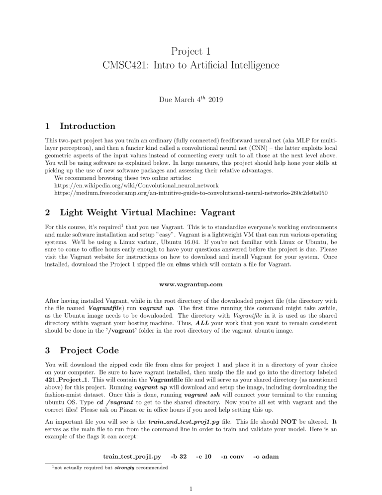
Project 1
CMSC421: Intro to Artificial Intelligence
Due March 4th 2019
1
Introduction
This two-part project has you train an ordinary (fully connected) feedforward neural net (aka MLP for multilayer perceptron), and then a fancier kind called a convolutional neural net (CNN) – the latter exploits local
geometric aspects of the input values instead of connecting every unit to all those at the next level above.
You will be using software as explained below. In large measure, this project should help hone your skills at
picking up the use of new software packages and assessing their relative advantages.
We recommend browsing these two online articles:
https://en.wikipedia.org/wiki/Convolutional neural network
https://medium.freecodecamp.org/an-intuitive-guide-to-convolutional-neural-networks-260c2de0a050
2
Light Weight Virtual Machine: Vagrant
For this course, it’s required1 that you use Vagrant. This is to standardize everyone’s working environments
and make software installation and setup ”easy”. Vagrant is a lightweight VM that can run various operating
systems. We’ll be using a Linux variant, Ubuntu 16.04. If you’re not familiar with Linux or Ubuntu, be
sure to come to office hours early enough to have your questions answered before the project is due. Please
visit the Vagrant website for instructions on how to download and install Vagrant for your system. Once
installed, download the Project 1 zipped file on elms which will contain a file for Vagrant.
www.vagrantup.com
After having installed Vagrant, while in the root directory of the downloaded project file (the directory with
the file named Vagrantfile) run vagrant up. The first time running this command might take awhile,
as the Ubuntu image needs to be downloaded. The directory with Vagrantfile in it is used as the shared
directory within vagrant your hosting machine. Thus, ALL your work that you want to remain consistent
should be done in the ’/vagrant’ folder in the root directory of the vagrant ubuntu image.
3
Project Code
You will download the zipped code file from elms for project 1 and place it in a directory of your choice
on your computer. Be sure to have vagrant installed, then unzip the file and go into the directory labeled
421 Project 1. This will contain the Vagrantfile file and will serve as your shared directory (as mentioned
above) for this project. Running vagrant up will download and setup the image, including downloading the
fashion-mnist dataset. Once this is done, running vagrant ssh will connect your terminal to the running
ubuntu OS. Type cd /vagrant to get to the shared directory. Now you’re all set with vagrant and the
correct files! Please ask on Piazza or in office hours if you need help setting this up.
An important file you will see is the train and test proj1.py file. This file should NOT be altered. It
serves as the main file to run from the command line in order to train and validate your model. Here is an
example of the flags it can accept:
train test proj1.py
1 not
-b 32
-e 10
actually required but strongly recommended
1
-n conv
-o adam
The -b flag is for the batch size the network uses when training/testing. The -e flag is for the number of
epochs the network will run when training (i.e. how many times does it run through the training data).
The -n flag determines what type of network to make: ’mlp’ for a fully connected network and ’conv’ for
a convolutional network. The -o flag is for what type of optimizer to use in training: ’sgd’ for stochastic
gradient descent, ’adam’ for adam, and ’rmsprop’ for rmsprop. There is a flag not shown , -s, that allows
for a snapshot of the weights of a network to be loaded back into the network. Snapshots are saved in the
snapshots directory. The name of a snapshot is specific to the date and time the network was created and
the type of network created. The history, named in a similar format, is also saved in order to continue the
plot created during training. This allows you to save a network after some training and go back and train it
further if you’d like. The history will also save the total training time to date and the current epoch, neither
of which you will have to manipulate as they will be automatically extracted from the history. If you use
the -s flag, the code will strip out the network type and the date of creation and continue training from the
last epoch number. After training, the total time for all training (which includes past episodes of training)
will be output. For instance, if you train your network and it takes 60 seconds, then you take a break and
two days later train the network some more and it takes 30 seconds, the total training time output after the
second training round will be 90 seconds. Finally, a -t flag can be used (as is, without any followup) in order
to just test the model you’re loading in with the -s flag. An accuracy score on the test set will be printed
out.
Note, there are two seeds set near the top of the model.py file. You can change the number used in these
to get di↵erent results; however, they are set such that you won’t get drastically inconsistent results when
running the same network (it’s possible the results may still di↵er ever so slightly). It’s ok (and good) to get
di↵erent results, but for your ease of comparing results in this class, the seeds have been fixed by default.
4
Fashion MNIST
This project will involve configuring a neural network that will learn to classify various images of clothing (e.g.
boot, sweater, etc.). The dataset we will be using is called Fashion MNIST which consists of greyscale
(only 1 color channel) images of various articles of clothing. The images are 28x28 (28x28x1 when including
the 1 color channel) in size and the features amongst some classes can be quite similar, making it difficult
even for humans to get 100% accuracy. A neural network can take advantage of statistical information
within the images, such as the likelihood of an image of a shoe having certain line arrangements or textures.
Although they pale in comparison to the whole of human visual capabilities and understanding, when it
comes to general object detection, neural networks have exceeded human accuracy for certain datasets 2 .
5
Keras and Tensorflow
We will be using a fairly simple frontend known as Keras that can use various neural network backends such
as Tensorflow, the Google-supported backend. One could simply roll their own neural network software,
but it’s much quicker, if not easier, to use a preexisting software such as Tensorflow. Others that exist and
are popular include Ca↵e (Facebook backed), PyTorch and Theano. We will be using Tensorflow as our
backend for consistency and legacy reasons.
6
Keras Tutorial
If you’ve successfully installed Vagrant and downloaded the files for this project, you should be all set to
start using Keras. Keras will have a Python implementation, allowing for use of the easy and widely used
Python scripting language to code neural networks. To gain a better understanding of how to use Keras in
your Python script, please see the Keras site https://keras.io. Otherwise, below are very quick examples
for a fully connected and a convolutional network.
If you’re unfamiliar with Python or need a reminder, # precedes comments per line. See the following
tutorial if you need a refresher:
https://docs.python.org/3/tutorial/
6.1
Coding Example: Fully Connected
2 Imagenet
for example
2
import k e r a s
from k e r a s . models import S e q u e n t i a l
from k e r a s . l a y e r s import Dense
# Convenient wrapper f o r c r e a t i n g a s e q u e n t i a l model
# where t h e o u t p u t o f one l a y e r f e e d s i n t o t h e i n p u t
# of the next layer .
model = S e q u e n t i a l ( )
#
#
#
#
#
#
#
#
” Dense ” h e r e i s t h e same as a f u l l y c o n n e c t e d network .
I n p u t dimension o n l y needs t o be s p e c i f i e d f o r t h e
f i r s t l a y e r , may be a t u p l e w i t h more than one
e n t r i e s , e . g . ( 1 0 0 , 1 0 0 , 3 ) f o r an i n p u t c o n s i s t i n g o f
c o l o r images ( RedBlueGreen s u b p i x e l s , hence t h e 3)
t h a t a r e 100 x100 p i x e l s i n s i z e . NOTE t h a t t h e
d a t a s e t we ’ l l be u s i n g has o n l y 1 c o l o r channel ,
NOT 3 l i k e i n t h i s example .
model . add ( Dense ( u n i t s =64 , a c t i v a t i o n= ’ r e l u ’ ,
i n p u t d i m =100))
model . add ( Dense ( u n i t s =10 , a c t i v a t i o n= ’ softmax ’ ) )
# S e t s up t h e model f o r t r a i n i n g and i n f e r r i n g .
model . compile ( l o s s= ’ c a t e g o r i c a l c r o s s e n t r o p y ’ ,
o p t i m i z e r= ’ sgd ’ ,
m e t r i c s =[ ’ a c c u r a c y ’ ] )
# The t r a i n i n g i s done here , c o u l d be b r o k e n up
# e x p l i c i t l y into batches .
model . f i t ( x t r a i n , y t r a i n , e p o c h s =5, b a t c h s i z e =32)
#
#
#
#
#
#
#
Get l o s s ( v a l u e o f l o s s f u n c t i o n , l o w e r i s b e t t e r )
and any m e t r i c s s p e c i f i e d i n t h e c o m p i l e s t e p ,
such as a c c u r a c y . The t e s t b a t c h c o n s i s t s o f h e l d o u t
d a t a t h a t you want t o v e r i f y your network on . You
s h o u l d NEVER use t e s t d a t a i n t h e t r a i n i n g p e r i o d . I t
v i o l a t e s s t a n d a r d s , e t h i c s and t h e c r e d i b i l i t y o f your
results .
l o s s a n d m e t r i c s = model . e v a l u a t e ( x t e s t , y t e s t ,
b a t c h s i z e =128)
# Get c l a s s o u t p u t s f o r t h e t e s t b a t c h s i z e o f 1 2 8 .
c l a s s e s = model . p r e d i c t ( x t e s t , b a t c h s i z e =128)
6.2
Coding Example: Convolutional
import k e r a s
from k e r a s . models import S e q u e n t i a l
from k e r a s . l a y e r s import Dense , F l a t t e n
from k e r a s . l a y e r s import Conv2D , MaxPooling2D
from k e r a s . o p t i m i z e r s import SGD
model = S e q u e n t i a l ( )
# i n p u t : 28 x28 images w i t h 1 c o l o r c h a n n e l > ( 2 8 , 28 , 1) t e n s o r s .
# t h i s a p p l i e s 32 c o n v o l u t i o n f i l t e r s o f s i z e 3 x3 each w i t h ’ r e l u ’
# a c t i v a t i o n a f t e r t h e c o n v o l u t i o n s a r e done .
3
model . add ( Conv2D ( 3 2 , ( 3 , 3 ) , a c t i v a t i o n= ’ r e l u ’ ,
i n p u t s h a p e =(28 , 2 8 , 1 ) ) )
model . add ( Conv2D ( 3 2 , ( 3 , 3 ) , a c t i v a t i o n= ’ r e l u ’ ) )
model . add ( MaxPooling2D ( p o o l s i z e =(2 , 2 ) ) )
model . add ( F l a t t e n ( ) )
model . add ( Dense ( 2 5 6 , a c t i v a t i o n= ’ r e l u ’ ) )
model . add ( Dropout ( 0 . 5 ) )
model . add ( Dense ( 1 0 , a c t i v a t i o n= ’ softmax ’ ) )
sgd = SGD( l r =0.01 , decay=1e 6, momentum=0.9 , n e s t e r o v=True )
model . compile ( l o s s= ’ c a t e g o r i c a l c r o s s e n t r o p y ’ , o p t i m i z e r=sgd )
# x t r a i n and y t r a i n not shown a b ov e . . . t h e s e
# a r e your i n p u t s and o u t p u t s f o r t r a i n i n g .
model . f i t ( x t r a i n , y t r a i n , b a t c h s i z e =32 , e p o c h s =10)
s c o r e = model . e v a l u a t e ( x t e s t , y t e s t , b a t c h s i z e =32)
CNNs add lots of subtle complexity of local spatial processing to nnets, in a way that often gains tremendous
efficiency. In the 2nd (convolutional) part of this project you are to play around with provided CNN code
(even if you don’t understand all the details) to see how much better your results on Fashion-MNIST can
be compared to a regular (non-CNN) nnet.
If you’ve browsed the suggested readings regarding convolutional neural networks (see above), you’ll notice
that there are some arguments missing that you might expect, such as padding. These arguments have
default settings. Padding for instance is set to ”valid” by default, meaning that there is no padding used and
the output of a convolutional layer will be smaller than that of its input (in the x-y direction, not necessarily
in the depth direction). The provided code gives you the basic framework above. It will be up to you to add
layers as necessary (within the guidelines outlined below).
7
Deliverables
For this project, you will use both a fully connected neural network and a convolutional neural network.
For the first part consisting solely of a fully connected network, no convolutional layers or other advanced
techniques are allowed. For the second part, both convolutional and fully connected layers are allowed but
NO other advanced techniques (ask if you’re not sure). You are only allowed to use the Fashion MNIST data
with NO augmentation of the data allowed. The examples above and the project code should provide you
with a large amount of the necessary information to implement a fully connected network and a convolutional
network. However, we’re leaving it up to you to further explore the Keras api via the provided site above
in regards to further details on the layers if necessary. This is an important part of learning how to utilize
existing frameworks for machine learning and AI.
The tasks to complete in specific are:
1. Fill in the layers of the skeleton fully connected neural network provided in the model.py file, in the
MLP function. At most 10 layers.
2. Fill in the layers of the skeleton convolutional neural network provided in the model.py file, in the
Conv function. At most 8 convolutional layers and 5 fully connected (FC) layers (not to be swapped!
e.g. no networks that are 10 convolutional layers and 3 FC layers or vice versa). Though note that
a max-pooling layer won’t count as a layer if you’re using those after the convolutional
layers. Again, ask if you’re unsure.
3. For three di↵erent network designs of each of the fully connected and the convolutional, include the
resulting plotted images of their accuracy and loss values per epoch. Be sure to indicate which network
design goes with which images.
4. Explain your network choices for the best networks for both fully connected and convolutional. Consider
factors such as speed of operation, accuracy, generalizability, etc. Also, discuss the di↵erences between
your fully connected and convolutional network results/performance. Give some reasons as to why you
think these di↵erences exist.
5. You will need to submit two files:
4
1.) the model.py file with your filled in networks (best performing ones). The submitted file should
be labeled <last name> <first name> model.py where <last name> and <first
name> are replaced with your actual last and first name, e.g. doe john model.py.
2.) pdf file containing the required explanations mentioned above in the project description. The
submitted file should be labeled <last name> <first name> analysis.pdf where
<last name> and <first name> are replaced with your actual last and first name,
e.g. doe john analysis.py.
5