Study Notes – Midterm BIOS 6100
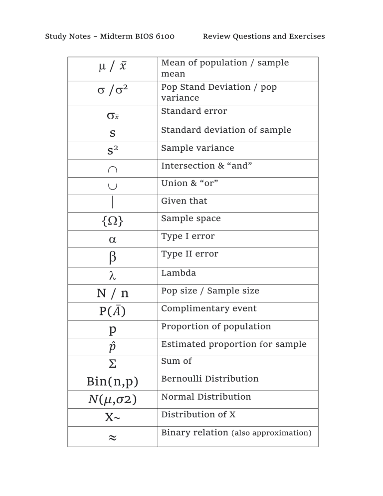
 / 𝑥̅
 /2
𝒙̅
s
s2



{}

β

N/n
P(𝐴̅)
p
𝑝̂
Σ
Bin(n,p)
N(μ,σ2)
X

Review Questions and Exercises
Mean of population / sample
mean
Pop Stand Deviation / pop
variance
Standard error
Standard deviation of sample
Sample variance
Intersection & “and”
Union & “or”
Given that
Sample space
Type I error
Type II error
Lambda
Pop size / Sample size
Complimentary event
Proportion of population
Estimated proportion for sample
Sum of
Bernoulli Distribution
Normal Distribution
Distribution of X
Binary relation (also approximation)
Chapter 1:
STATISTICS: A field of study concerned with (1) the collection, organization,
summarization and analysis of data; and (2) the drawing of inferences
about a body of data when only a part of the data is observed.
1. Explain what is meant by descriptive statistics.
Descriptive statistics summarize data, inferential statistics help you come
to conclusions and make predictions based on your data.
Descriptive statistics are used measure to data through:




Measures of
Measures of
Measures of
Deviation.
Measures of
Frequency: * Count, Percent, Frequency.
Central Tendency. * Mean, Median, and Mode.
Dispersion or Variation. * Range, Variance, Standard
Position. * Percentile Ranks, Quartile Ranks.
2. What is meant by inferential statistics?
The inferences and conclusions gathered from descriptive stats to
make predictions on the general population based on sample data.



Hypothesis testing
Confidence interval
Regression analysis
3. DEFINE:
(a) Biostatistics: the application of statistical techniques to scientific
research in health-related fields, including medicine, biology, and
public health.
(b) Variable: observable characteristics that takes on different values in
different people, places, things.
(c) Quantitative variable: a characteristic in the usual sense, can be
measured.
(d) Qualitative variable: Some characteristics cannot be measured like
we can with quantitative variables like age, weight, etc., but they can be
categorized such as healthy or ill, ethnicities, gender, etc.
(e) Random variable: (value of a respective variable) – when values are
obtained due to chance factors, cannot be predicted in advance. (Adult
height w/babies)
(f) Population: A population of entities as the largest collection of entities
for which we have an interest at a particular time.
(g) Finite population: possible to count individuals (countable: births
per year).
(h) Infinite population: A population that consists of endless succession
of values.
(i) Sample: part of a population – representative of the group in some
form.
(j) Discrete variable: (not continuous) – characterized by gaps or
interruptions in the values that it can assume.  absence of values,
whole #s (hospital admissions, teeth filled per child in an elementary
school, etc.)
Continuous variable: a continuous random variable does not possess
gaps or interruptions characteristic of a discrete random variable.
(weight, height, there is always someone that can fit b/t two samples.
Tools are problem to measure.
(k) Simple random sample: Random selection of subgroup from pop.
Each member of the population has an equal chance of being selected.
Simplest form.
(l) Sampling without replacement: each sample unit of the population
has only one chance to be selected in the sample.
(m) Sampling w/Replacement: the selected person gets put back in pop
after being selected.
4. Define the word measurement: Defined as the assignment of numbers
to objects or events according to a set of rules. Carried under diff set
of rules.
5. Define and describe the 4 measurement scales.
(a) Nominal scale: names – male/female, ill/healthy, under 18/over
18, adult/child, married/not married, etc.
(b) Ordinal scale: Order – convalescing: unimproved, improved, +
improved
(c)
Interval scale: use of a unit distance and a zero point is not true
zero, like the weather (degrees)
(d)
Ratio scale: highest level of measurement. Equality of ratios and
equality of intervals may be determined. “True zero point”- height,
weight, length.
6. For each of the following variables, indicate whether it is quantitative
or qualitative and specify the measurement scale that is employed
when taking measurements of each:
(a) Class standing of the members of this class relative to each
other:
 Ordinal scale: qualitative
(b) Admitting diagnosis of patients admitted to a mental health
clinic:
 Ordinal scale: qualitative
(c) Weights of babies born in a hospital during a year:
 ratio scale: quantitative
(d) Gender of babies born in a hospital during a year:
 Nominal scale: qualitative
(e)Range of motion of elbow joint of students enrolled in a university
HS course
interval scale: qualitative
(f) Under-arm temperature of day-old infants born in a hospital:
 interval scale: quantitative
7. For each of the following situations, answer question a – e
(a)
What is the sample in the study?
A  300 households made up the sample
B 250 patients admitted in past year
(b)
What is the population?
A  The 20% of the participating households of the town w/children
B  Patients admitted to hospital in last year
(c) What is the variable of interest?
A  families that have school-age children
B  Distance from hospital
(d)
How many measurements were used in calculating the reported
results?
A  Nominal scale and ratio scale for school-aged children,
quantitative
B
(e)What measurement scale:
A  ratio and nominal
B  Ratio Scale – distance
8. A: Describe how you would use a stratified random sample to collect
the data
(proportional random sampling) Probability sampling technique in
which the total population is divided into homogenous sub-groups
(strata) based on specific characteristics (gender, race, location, etc.)
to complete the sampling process. Every member of the population
studied should be in exactly one stratum. Used for diverse populations
to ensure that every characteristic is properly represented.
 I would subdivide the families with children into age categories,
race, gender, SES, etc.
B: Use systematic sampling of patient records to collect the data
Choosing a sampling method at random, but with a predetermined
starting point. For instance choosing every 10th employee, or 7th
student on a list. Preferred to simple random sample if there is low
risk of manipulation. For example 50 participants are needed and you
have a group of 500 people, then every 10th person would be a good
choice.
 Chose every 5th patient to fill questionnaire on dwelling location, or
use databank and pull every 9th patient..
Chapter 2:
1. Define:
(a)
Stem-and-leaf-display: Resembles a histogram and serves the
same purpose. Provides information on range of data set, shows
location of the highest concentration of measurements, reveals
absence/presence of symmetry. *Small amounts of data.
 Each data value is split into a “steam” and a “leaf”, meaning the main
number (tens (decenas)hundreds, etc.) are on the left as the stem, and on
right, under leaf are the unidades.
(b)
Box-and-whisker plot: (boxplot) uses quartiles data set.
It is a method for graphically demonstrating the locality, spread and
skewness groups of numerical data through their quartiles.
5 points are needed: min value, max value, Q1, Q2, & Q3
Find the inter-quartile range (IQR) which is the subtraction of Q3-Q1 and
figure out if there are outliers (Q1 – 1.5) IQR AND Q3 +1.5 * IQR, then
plot
(c) Percentile: a value on a scale of 100 that indicates the percent of a
distribution that is equal to or below it a score in the 95th
percentile.
(d) Quartile: each of 4 equal groups that a pop can be divided into given
particular values of a variable.
(e)Location parameter: tells you where your graph is located. More
specifically, it tells you where on the horizontal axis a graph is
centered, relative to the standard normal model.
(f) Exploratory data analysis: refers to the critical process of performing
initial investigations on data so as to discover patterns, to spot
anomalies, to test hypothesis and to check assumptions with the
help of summary statistics and graphical representations.
BOXPLOTS, STEM & LEAF
(g)
Ordered array: The elements of an ordered array are arranged
in ascending (or descending) order.
(h) Frequency distribution: a mathematical function showing the number
of instances in which a variable takes each of its possible values.
(i) Relative frequency distribution: A relative frequency
distribution shows the proportion of the total number of
observations associated with each value or class of values and is
related to a probability distribution.
(j) Statistics: are defined as numerical data, and is the field of math that
deals with the collection, tabulation and interpretation of numerical
data FROM A SAMPLE.
(k)
Parameter: a parameter is any measured quantity of a statistical
population that summarizes or describes an aspect of the population, such as a
mean or a standard deviation.
(l) Frequency polygon: is a graphical form of representation of data. It
is used to depict the shape of the data and to depict trends. It is
usually drawn with the help of a histogram but can be drawn without
it as well.
(m)
True class limits –
(n)
Histogram: an approximate representation of the distribution of
numerical data.
2. Mean, Median and mode –
3. + and – of range as a measure of dispersion: the difference between the
largest and the smallest observation in the data. The prime advantage
of this measure of dispersion is that it is easy to calculate. On the other
hand, it has lot of disadvantages. It is very sensitive to outliers and does
not use all the observations in a data set.
4. We use n-1 when calculating sample variance to try to diminish the
sample bias because the sample mean tends to sit within the sample, and
perhaps not that of the overall mean of the population; to the point that
the population mean could be outside of the sample. Which could lead to
underestimating the true population variance. The n-1 yields a larger
sample variance = less biased.
5. What is the purpose of the coefficient of variation (CV)? To compare
results from two different tests or data sets that have different measures
or values. *diff scoring mechanisms
6. What is the purpose of Sturge’s rule?
- Use for continuous data, normally distributed and symmetrical
7. Second or middle quartile or 50th percentile is the median (and the mean
in a normal distribution).
CHAPTER 3
1. Define
(a) Probability: the extent to which something is probable; the likelihood
of something happening or being the case.
(b) Objective probability: refers to the chances or the odds that an event
will occur based on the analysis of concrete measures rather than
hunches or guesswork. Each measure is a recorded observation, a
fact, or part of a long history of collected data.
(c)
Subjective probability: derived from personal judgement or
experience.
(d)
(e)
(f)
(g)
(h)
(i)
Classical probability: dates to 17th century for games of chance
The relative frequency of probability: the ratio of the number of
outcomes in which a specified event occurs to the total number or
trials, not in a theoretical sample space, but in an actual experiment.
Mutually exclusive events: two or more events that CANNOT happen
simultaneously. Heads/Tails in coin tosses.
Independence: the occurrence of one event does not affect the
probability of the occurrence of the other.
Conditional probability: (Bayes’ theorem & Tree diagrams). The
probability of an event occurring, given that another event has already
occurred. The likelihood of an outcome occurring, based on the
occurrence of a previous event or outcome. P(A∪B) event A happening
and event B happening.
P(A|B) – the conditional probability; the probability of event A
occurring given that event B has already occurred.
Joint probability: P(A ⋂ B) = P(A) x P(B). Probability that two event
will both occur. Joint probability is the likelihood of two events
occurring together, but not due to one another. Events are
independent, so events cannot influence outcome of each other. Think
rolling a 5 twice in a fair six-sided dice.
(j)
Marginal probability: event will occur irrespective of the outcome of
another variable = Red card from deck: ½ chance and a number 4 card
is 1/13.
(k)
The addition rule: If A and B are two events in a probability
experiment, then the probability that either one of the events will
occur is:
P (A or B) = P(A)+P(B) — P (A and B).
(l)
The multiplication rule: Rule in probability that allows to calculate the
probability of multiple events occurring together using known
probabilities of those events individually.
(m)
Complementary events: One event occurs if and only if the other does
not. Two Complementary events add up to 1.
P(A) + P(Ā) = 1  P(Ā) = 1— P(A)  P(A) = 1— P(Ā)
(n)
False Positive: Type 1 error – incorrectly test + when disease is absent.
(o)
False negative: Type 2 error – test is negative when disease is present.
(p)
Sensitivity: percentage of true positives –
(q)
Specificity: percentage of true negatives –
(r)
Predictive value positive (PV+) – ratio of patients truly diagnosed as
positive to all those who had a positive test.
(s)
Predictive value negative (PV-): ratio of the subjects diagnosed as
negative to all those who had negative test results.
Baye’s Theorem: is a formula to predict the probability that a given cause
was responsible for an observed outcome - assuming that the probability of
observing that outcome for every possible cause is known, and that all causes
and events are independent.
However, the positive and negative predictive values can also be obtained by
simple algebraic rearrangement of the terms in the 2-by-2 table.
(t)
describes the probability of an event, based on prior knowledge of
conditions that might be related to the event.
Name and explain the 3 properties of probability:
0 and 1 measure the likelihood of the occurrence of some event
-
All events must have a probability greater than or equal to zero.
-
Mutually exclusive outcomes – cannot occur simultaneously
-
The sum of the probabilities of the mutually exclusive outcomes
equals to 1  exhaustiveness – all probabilities when done = 1
-
Two mutually exclusive events Ei and Ej is equal to the sum of their
individual probabilities.