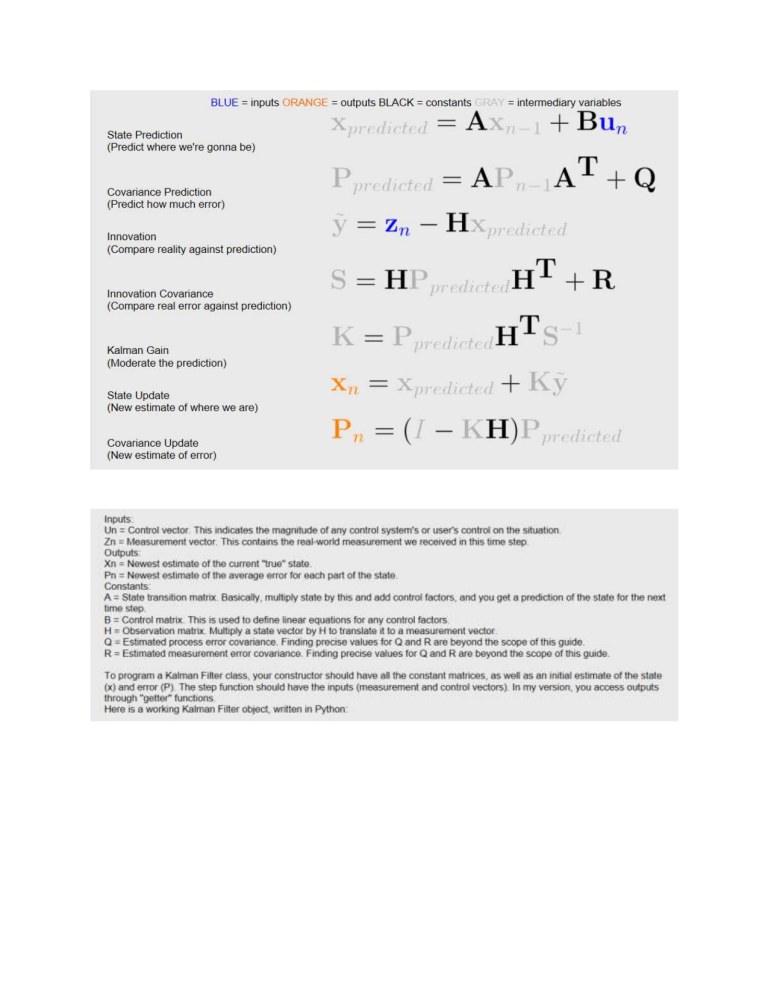
Part I - Who is Who in the Land of Kalman Filters
Oh my gosh, you say, what the heck are all those Kalman matrices and vectors? I have no idea
what's going on, you say. Sebastian kind of threw them at us without a whole lot of explanation. Ok,
well, let's try to figure them out a bit. Capital letters are for 2-D matrices, and bold lower case are for
vectors, which are 1-D matrices.
VECTOR X, THE VARIABLES
x is the values of all the variables you're considering in your system. It might, for example, be
position and velocity. Or if you were using a Kalman filter to model polling results, it might be Rick
Santorum's support and momentum in Ohio Presidential polls. It might be a sick person's
temperature and how fast the temperature is going up. It's a vector. Let's say it has n elements —
that will be important for the size of other matrices.
For example, let's say we're modeling a sick person's temperature. She's lying there in the hospital
bed with three temperature sensors stuck to her, and we want to see if her temperature is going up
fast, in which case we'll call a nurse. (For purposes of this example, we'll assume that in the time
period we're observing, the rate of rise is constant.)
We might initialize x with a temperature of 98.6 and a temperature rising rate of 0. The Kalman filter
algorithm will change x--that's the whole point, to find the correct values for x.
MATRIX F, THE UPDATE MATRIX
F is the n by n update matrix. Kalman filters model a system over time. After each tick of time, we
predict what the values of x are, and then we measure and do some computation. F is used in the
update step. Here's how it works: For each value in x, we write an equation to update that value, a
linear equation in all the variables in x. Then we can just read off the coefficients to make the matrix.
For our example, our x vector would be (x1, x2) where x1 is the temperature in degrees and x2 is the
rate of change in hundredths of a degree (doesn't matter whether Celsius or Fahrenheit, just as long
as it's the same for all) per minute. We check our sensors every minute, and update every minute.
Let's figure out how to make the matrix F. If our patient's temperature is x1, what is it one minute
later? It's x1, the old temperature, plus the change. Note that because temperature is in degrees but
the change is in hundredths of degrees, we have to put in the coefficient of 1/100.

x[1]' = x[1] + x[2]/100
If the rate of change is x2, what is it one minute later? Still x2, because we've assumed the rate is
constant.

x[2]' = 0x[1] + x[2]
Now we write out all our equations, like this:


x[1]' = x[1] + x[2]/100
x[2]' = 0x[1] + x[2]
In words, the new temperature, x1', is the old temperature plus the rise over the time segment. The
new rate of change, x2', is the same as the old rate of change. We can just read off the coefficients
of the right hand side, and there's our matrix F:


1 .01
01
Bingo. Note that these equations have to be linear equations in the variables. We might want to take
the sine of a variable, or square it, or multiply two variables together. We can't, though, not in a
Kalman filter. These are linear equations.
Z, THE MEASUREMENT VECTOR
Now let's turn to z, the measurement vector. It's just the outputs from the sensors. Simple. Let's say
we have m sensors. That could be, and probably is, different from n, the number of variables we're
keeping track of. In our example, let's say we have three temperature probes, all somewhat
inaccurate.
H, THE EXTRACTION MATRIX
The matrix H tells us what sensor readings we'd get if x were the true state of affairs and our sensors
were perfect. It's the matrix we use to extract the measurement from the data. If we multiply H times
a perfectly correct x, we get a perfectly correct z.
So let's figure out what z1, z2 and z3, the readings from our three temperature sensors, would be if
we actually knew the patient's temperature and rate of temperature rising, and our sensors were
perfect. Again, we just write out our equations:



z1 = x1 + 0x2
z2 = x1 + 0x2
z3 = x1 + 0x2
because if we knew the patients real temperature, and our sensors perfectly measured that
temperature, z1 would be the same as x1 and so would z2 and z3. Again, we just read off the
coefficients to make H:



10
10
10
Remember F, the update matrix, is n by n. Notice that H, the extraction matrix, is m by n. When we
multiply H by x, we get a vector of size m.
P, THE COVARIANCE MATRIX OF X
P is the covariance matrix of the vector x. x is a vector of dimension n, so P is n by n. Down the
diagonal of P, we find the variances of the elements of x: the bigger the number, the bigger our
window of uncertainty for that element. On the off diagonals, at P[i][j], we find the covariances of x[i]
with x[j]. Covariance matrices must be symmetric matrices, because the covariance of x[i] and x[j] is
also the covariance of x[j] and x[i], so P[i][j]==P[j][i]. That is, the whole thing is symmetric down the
main diagonal.
P gets updated as we run our Kalman filter and become more certain of the value of the x vector.
For the patient example, we start out pretty uncertain. We'll give pretty big variances to both x1, the
temperature, and x2, the rate of change in temperature. We don't have any notion that temperature
and rise in temperature are correlated, so we'll make the covariance 0. So the matrix will look like

30

0 .1
R, THE COVARIANCE MATRIX OF THE MEASUREMENT VECTOR Z
R is also a covariance matrix, but it's the variances and covariances of our sensor measurements.
Because z has dimension m, R is an m by m matrix. The Kalman filter algorithm does not change R,
because the process can't change our belief about the accuracy of our sensors--that's a property of
the sensors themselves. We know the variance of our sensor either by testing it, or by reading the
documentation that came with it, or something like that. Note that the covariances here are the
covariances of the measurement error. A positive number means that if the first sensor is
erroneously low, the second tends to be erroneously low, or if the first reads high, the second tends
to read high; it doesn't mean that if the first sensor reports a high number the second will also report
a high number.
In our patient example, the three sensors are measuring exactly the same thing. So of course, their
readings will be correlated. But, let's say that any two sensors don't tend to be off the same way-- the
inaccuracy is caused by cheap manufacturing techniques, not by something about the patient. In
that case, we'd give them covariances of zero. Our sensors, let's say, have variances of .2; they're
not very accurate. So our covariance matrix might look like:



.2 0 0
0 .2 0
0 0 .2
But if we knew that the measurements from the three sensors tended to be off in the same direction-maybe all of them read low if a fan is blowing in the room, and high if music is playing--then we'd
put positive covariances for them:



.2 .05 .05
.05 .2 .05
.05 .05 .2
U, THE MOVE VECTOR
The last input matrix is the vector u. This one is pretty simple; it's the control input, the move vector.
It's the change to x that we cause, or that we know is happening. Since we add it to x, it has
dimension n. When the filter updates, it adds u to the new x.
I can't think of a good example using our patient and our thermometers, but suppose we were
modeling the location and velocity of an object, and in addition to watching it move, we could also
give it a shove. In the prediction stage, we'd update the object's location based on our velocity, but
then with u we'd add to its position and velocity because we moved it. u can change for each
iteration of the Kalman filter. In our examples in class, it's always all zeros; we're not moving
anything ourselves, just watching it move.
This is part I of an explanation of all the matrices in the Kalman filter. I'm writing it up for myself to
see if I understand what's going on. This is very much a work in progress and needs proofreading.
Part II (sketchy right now) covers S, K and y. Part III has some general comments about how the
Kalman filter works, what kind of problems it works for, and what kind of problems it doesn't work for.
Part II - How It Works
This post describes the Kalman filter process as I understand it. I noticed, to my surprise, that P, our
covariance matrix, never depends on the observed values z or the move u,so the Kalman filter
converges in the same number of steps, possibly an infinite number, no matter what we observe.
(Thank you to @kpalamartchouk.) As @amorfis points out below in the comments, just as with
combining one dimensional gaussians, the new variance is a function of the old variances but not
the old means.
PREDICT X'
First, we predict our next x:
x' = Fx + u
UPDATE P'
P is the expectation of x times (transp x). We update it to be the expectation of Fx times (transp Fx):
P' = Fx*(trans Fx)
UPDATE Y
y becomes the difference between the move and what we expected:
y = z - Hx
UPDATE S
S is the covariance of the move, adding up the covariance in move space of the position and the
covariance of the measurement:
S = HP(transp H) + R
CALCULATE K
Now I start to wave my hands. I assume this next matrix is called K because this is the work of the
Kalman filter. Whatever is happening here, it doesn't depend on u or z. We're computing how much
of the difference between the observed move and the expected move to add to x.
K = P (transp H) (inv S)
UPDATE X'
We update x:
x' = x + Ky
SUBTRACT P
And we subtract some uncertainty from P, again not depending on u or z:
P' = P - P(transp H)(inv S)HP
Our input doesn't affect how fast we converge.
Part III - When it Works and When It Does Not Work
In this post I'll just say a few things about how the filter works and when it doesn't. With a Kalman
filter, we have a bunch of state variables (in the class example they were position and velocity) and
some sensors that give us information about the variables (in the class, one location sensor).
Crucially, the bunch of variables have to be unimodal, which means that we have one belief,
although perhaps an uncertain one, about the values of the variables. Our sensor inputs are
unimodal too
That is, we can represent the notion that the car is over there, about 12 meters away but maybe as
close as 9 meters or as far away as 15 meters. But we can't represent the belief that the car might
be over there to the left, around 12 meters away, or else maybe I was looking in a mirror and it was
actually over there to the right, around 12 meters away. Think back to the last class, where the robot
saw a door and was pretty sure it was either in front of door #1, or door #2, or door #3. The Kalman
filter can't handle that at all. The particle filter that we're about to learn about does wonderfully with
that sort of belief, but the Kalman filter does not.
Both the sensor input and the belief about the state variables have to be not only unimodal, but
gaussian. The Kalman filter update is, essentially, multiplying two gaussians just like we did in class,
but since they are multivariate (more than one variable) gaussians it has to get smart about doing
the right thing with correlations. (If you have two sensors that both tend to be wrong in the same
direction, you shouldn't take the second one as strong confirmation of the first one, and the linear
algebra in the Kalman equations handles that.) The Kalman equations do operations that are only
valid if the sensors and state are gaussian-- otherwise, the filter is just doing meaningless
mathematical operations that might or might not come up with plausible numbers.
Here's the non-intuitive result: the P matrix shows the variances of your state variables in its
diagonals. Small numbers there represent more certainty that the state variables are close to their
true values. Those numbers are going to get smaller and smaller as you do more cycles
independent of your sensor measurements! That is, whatever your sensor sees, you'll get more and
more certain that your state variables are correct in exactly the same way.
So, bottom line, for a Kalman filter model to work, you need




some state variables where your belief about them forms a gaussian (though you can cheat
and start with such a wide gaussian that it's rather like a uniform distribution)
some linear equations in your state variables that transform your state variables into new state
variables with no uncertainty
some sensor outputs which are gaussian
the variances and covariances of your sensor outputs