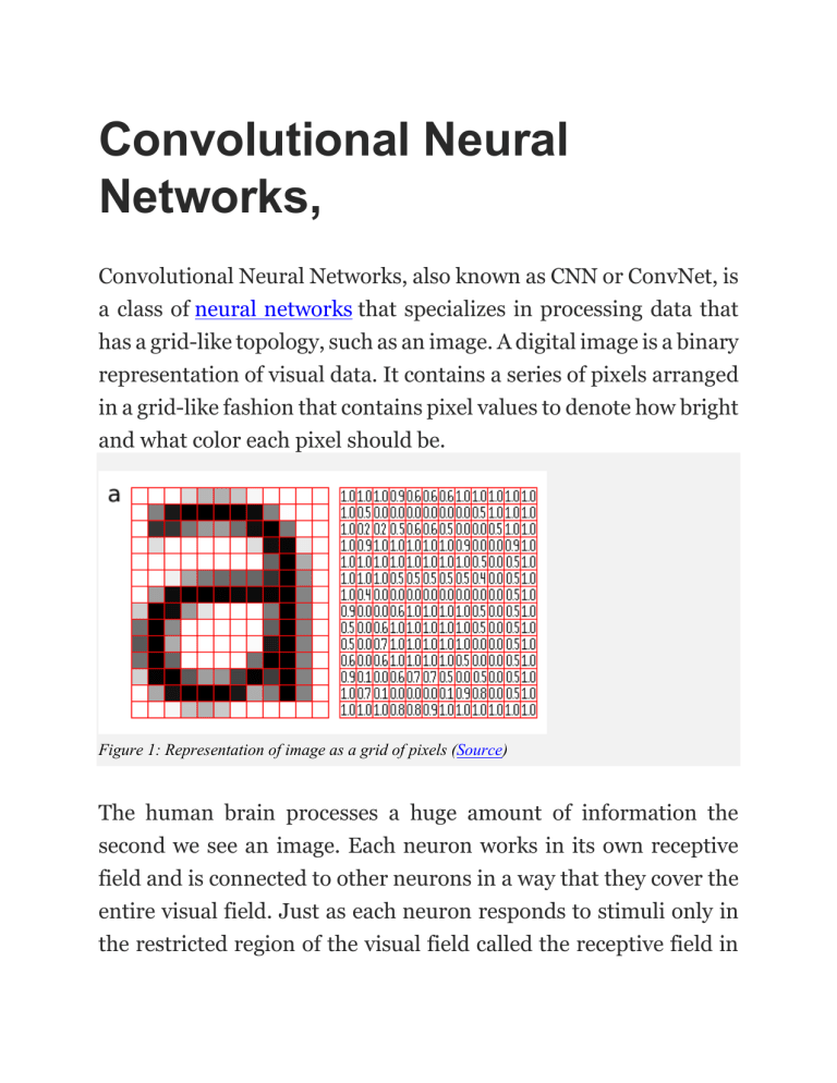
Convolutional Neural
Networks,
Convolutional Neural Networks, also known as CNN or ConvNet, is
a class of neural networks that specializes in processing data that
has a grid-like topology, such as an image. A digital image is a binary
representation of visual data. It contains a series of pixels arranged
in a grid-like fashion that contains pixel values to denote how bright
and what color each pixel should be.
Figure 1: Representation of image as a grid of pixels (Source)
The human brain processes a huge amount of information the
second we see an image. Each neuron works in its own receptive
field and is connected to other neurons in a way that they cover the
entire visual field. Just as each neuron responds to stimuli only in
the restricted region of the visual field called the receptive field in
the biological vision system, each neuron in a CNN processes data
only in its receptive field as well. The layers are arranged in such a
way so that they detect simpler patterns first (lines, curves, etc.) and
more complex patterns (faces, objects, etc.) further along. By using
a CNN, one can enable sight to computers.
Convolutional Neural Network Architecture
A CNN typically has three layers: a convolutional layer, a pooling
layer, and a fully connected layer.
Figure 2: Architecture of a CNN (Source)
Convolution Layer
The convolution layer is the core building block of the CNN. It
carries the main portion of the network’s computational load.
This layer performs a dot product between two matrices, where
one matrix is the set of learnable parameters otherwise known as a
kernel, and the other matrix is the restricted portion of the
receptive field. The kernel is spatially smaller than an image but is
more in-depth. This means that, if the image is composed of three
(RGB) channels, the kernel height and width will be spatially
small, but the depth extends up to all three channels.
Illustration of Convolution Operation (source)
During the forward pass, the kernel slides across the height and
width of the image-producing the image representation of that
receptive region. This produces a two-dimensional representation
of the image known as an activation map that gives the response of
the kernel at each spatial position of the image. The sliding size of
the kernel is called a stride.
If we have an input of size W x W x D and Dout number of kernels
with a spatial size of F with stride S and amount of padding P, then
the size of output volume can be determined by the following
formula:
Formula for Convolution Layer
This will yield an output volume of size Wout x Wout x Dout.
Figure 3: Convolution Operation (Source: Deep Learning by Ian Goodfellow, Yoshua Bengio,
and Aaron Courville)
Motivation behind Convolution
Convolution leverages three important ideas that motivated
computer vision researchers: sparse interaction, parameter
sharing, and equivariant representation. Let’s describe each one of
them in detail.
Trivial neural network layers use matrix multiplication by a matrix
of parameters describing the interaction between the input and
output unit. This means that every output unit interacts with every
input unit. However, convolution neural networks have sparse
interaction. This is achieved by making kernel smaller than the
input e.g., an image can have millions or thousands of pixels, but
while processing it using kernel we can detect meaningful
information that is of tens or hundreds of pixels. This means that
we need to store fewer parameters that not only reduces the
memory requirement of the model but also improves the statistical
efficiency of the model.
If computing one feature at a spatial point (x1, y1) is useful then it
should also be useful at some other spatial point say (x2, y2). It
means that for a single two-dimensional slice i.e., for creating one
activation map, neurons are constrained to use the same set of
weights. In a traditional neural network, each element of the weight
matrix is used once and then never revisited, while convolution
network has shared parameters i.e., for getting output, weights
applied to one input are the same as the weight applied elsewhere.
Due to parameter sharing, the layers of convolution neural network
will have a property of equivariance to translation. It says that if
we changed the input in a way, the output will also get changed in
the same way.
Pooling Layer
The pooling layer replaces the output of the network at certain
locations by deriving a summary statistic of the nearby outputs.
This helps in reducing the spatial size of the representation, which
decreases the required amount of computation and weights. The
pooling operation is processed on every slice of the representation
individually.
There are several pooling functions such as the average of the
rectangular
neighborhood,
L2
norm
of
the
rectangular
neighborhood, and a weighted average based on the distance from
the central pixel. However, the most popular process is max
pooling,
which
reports
the
maximum
neighborhood.
Figure 4: Pooling Operation (Source: O’Reilly Media)
output
from
the
If we have an activation map of size W x W x D, a pooling kernel of
spatial size F, and stride S, then the size of output volume can be
determined by the following formula:
Formula for Padding Layer
This will yield an output volume of size Wout x Wout x D.
In all cases, pooling provides some translation invariance which
means that an object would be recognizable regardless of where it
appears on the frame.
Fully Connected Layer
Neurons in this layer have full connectivity with all neurons in the
preceding and succeeding layer as seen in regular FCNN. This is
why it can be computed as usual by a matrix multiplication followed
by a bias effect.
The FC layer helps to map the representation between the input and
the output.
Non-Linearity Layers
Since convolution is a linear operation and images are far from
linear, non-linearity layers are often placed directly after the
convolutional layer to introduce non-linearity to the activation
map.
There are several types of non-linear operations, the popular ones
being:
1. Sigmoid
The sigmoid non-linearity has the mathematical form σ(κ) =
1/(1+e¯κ). It takes a real-valued number and “squashes” it into a
range between 0 and 1.
However, a very undesirable property of sigmoid is that when the
activation is at either tail, the gradient becomes almost zero. If the
local gradient becomes very small, then in backpropagation it will
effectively “kill” the gradient. Also, if the data coming into the
neuron is always positive, then the output of sigmoid will be either
all positives or all negatives, resulting in a zig-zag dynamic of
gradient updates for weight.
2. Tanh
Tanh squashes a real-valued number to the range [-1, 1]. Like
sigmoid, the activation saturates, but — unlike the sigmoid neurons
— its output is zero centered.
3. ReLU
The Rectified Linear Unit (ReLU) has become very popular in the
last few years. It computes the function ƒ(κ)=max (0,κ). In other
words, the activation is simply threshold at zero.
In comparison to sigmoid and tanh, ReLU is more reliable and
accelerates the convergence by six times.
Unfortunately, a con is that ReLU can be fragile during training. A
large gradient flowing through it can update it in such a way that
the neuron will never get further updated. However, we can work
with this by setting a proper learning rate.
Designing a Convolutional Neural Network
Now that we understand the various components, we can build a
convolutional neural network. We will be using Fashion-MNIST,
which is a dataset of Zalando’s article images consisting of a training
set of 60,000 examples and a test set of 10,000 examples. Each
example is a 28x28 grayscale image, associated with a label from 10
classes. The dataset can be downloaded here.
Our convolutional neural network has architecture as follows:
[INPUT]
→[CONV 1] → [BATCH NORM] → [ReLU] → [POOL 1]
→ [CONV 2] → [BATCH NORM] → [ReLU] → [POOL 2]
→ [FC LAYER] → [RESULT]
For both conv layers, we will use kernel of spatial size 5 x 5 with
stride size 1 and padding of 2. For both pooling layers, we will use
max pool operation with kernel size 2, stride 2, and zero padding.
Calculations for Conv 1 Layer (Image by Author)
Calculations for Pool1 Layer (Image by Author)
Calculations for Conv 2 Layer (Image by Author)
Calculations for Pool2 Layer (Image by Author)
Size of Fully Connected Layer (Image by Author)
Code snipped for defining the convnet
class convnet1(nn.Module):
def __init__(self):
super(convnet1, self).__init__()
# Constraints for layer 1
self.conv1 = nn.Conv2d(in_channels=1, out_channels=16,
kernel_size=5, stride = 1, padding=2)
self.batch1 = nn.BatchNorm2d(16)
self.relu1 = nn.ReLU()
self.pool1 = nn.MaxPool2d(kernel_size=2) #default stride is
equivalent to the kernel_size
# Constraints for layer 2
self.conv2 = nn.Conv2d(in_channels=16, out_channels=32,
kernel_size=5, stride = 1, padding=2)
self.batch2 = nn.BatchNorm2d(32)
self.relu2 = nn.ReLU()
self.pool2 = nn.MaxPool2d(kernel_size=2)
# Defining the Linear layer
self.fc = nn.Linear(32*7*7, 10)
# defining the network flow
def forward(self, x):
# Conv 1
out = self.conv1(x)
out = self.batch1(out)
out = self.relu1(out)
# Max Pool 1
out = self.pool1(out)
# Conv 2
out = self.conv2(out)
out = self.batch2(out)
out = self.relu2(out)
# Max Pool 2
out = self.pool2(out)
out = out.view(out.size(0), -1)
# Linear Layer
out = self.fc(out)
return out
We have also used batch normalization in our network, which saves
us from improper initialization of weight matrices by explicitly
forcing the network to take on unit Gaussian distribution. The code
for the above-defined network is available here. We have trained
using cross-entropy as our loss function and the Adam Optimizer
with a learning rate of 0.001. After training the model, we achieved
90% accuracy on the test dataset.
Applications
Below are some applications of Convolutional Neural Networks
used today:
1. Object detection: With CNN, we now have sophisticated models
like R-CNN, Fast
R-CNN,
and Faster
R-CNN that
are
the
predominant pipeline for many object detection models deployed
in autonomous vehicles, facial detection, and more.
2. Semantic segmentation: In 2015, a group of researchers from
Hong Kong developed a CNN-based Deep Parsing Network to
incorporate rich information into an image segmentation model.
Researchers from UC Berkeley also built fully convolutional
networks that
improved
upon
state-of-the-art
semantic
segmentation.
3. Image captioning: CNNs are used with recurrent neural networks
to write captions for images and videos. This can be used for many
applications such as activity recognition or describing videos and
images for the visually impaired. It has been heavily deployed by
YouTube to make sense to the huge number of videos uploaded to
the platform on a regular basis.
References
1. Deep Learning by Ian Goodfellow, Yoshua Bengio and Aaron
Courville published by MIT Press, 2016
2. Stanford University’s Course — CS231n: Convolutional Neural
Network for Visual Recognition by Prof. Fei-Fei Li, Justin Johnson,
Serena Yeung
3. https://datascience.stackexchange.com/questions/14349/differ
ence-of-activation-functions-in-neural-networks-in-general
4. https://www.codementor.io/james_aka_yale/convolutionalneural-networks-the-biologically-inspired-model-iq6s48zms
5. https://searchenterpriseai.techtarget.com/definition/convoluti
onal-neural-network