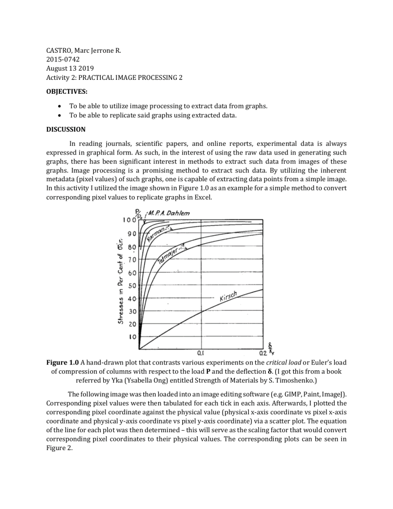
CASTRO, Marc Jerrone R.
2015-0742
August 13 2019
Activity 2: PRACTICAL IMAGE PROCESSING 2
OBJECTIVES:
•
•
To be able to utilize image processing to extract data from graphs.
To be able to replicate said graphs using extracted data.
DISCUSSION
In reading journals, scientific papers, and online reports, experimental data is always
expressed in graphical form. As such, in the interest of using the raw data used in generating such
graphs, there has been significant interest in methods to extract such data from images of these
graphs. Image processing is a promising method to extract such data. By utilizing the inherent
metadata (pixel values) of such graphs, one is capable of extracting data points from a simple image.
In this activity I utilized the image shown in Figure 1.0 as an example for a simple method to convert
corresponding pixel values to replicate graphs in Excel.
Figure 1.0 A hand-drawn plot that contrasts various experiments on the critical load or Euler’s load
of compression of columns with respect to the load P and the deflection δ. (I got this from a book
referred by Yka (Ysabella Ong) entitled Strength of Materials by S. Timoshenko.)
The following image was then loaded into an image editing software (e.g. GIMP, Paint, ImageJ).
Corresponding pixel values were then tabulated for each tick in each axis. Afterwards, I plotted the
corresponding pixel coordinate against the physical value (physical x-axis coordinate vs pixel x-axis
coordinate and physical y-axis coordinate vs pixel y-axis coordinate) via a scatter plot. The equation
of the line for each plot was then determined – this will serve as the scaling factor that would convert
corresponding pixel coordinates to their physical values. The corresponding plots can be seen in
Figure 2.
Physical Y-Coordinate vs Pixel Y-Coordinate
Physical Y Coordinate
120
100
80
y = -0.2329x + 110.68
60
40
20
0
0
100
200
300
400
500
Pixel Y Coordinate
Physical X-Coordinate vs Pixel X-Coordinate
Physical x Coordinate
0.25
0.2
y = 0.0005x - 0.0392
0.15
0.1
0.05
0
0
100
200
300
400
500
600
Pixel x Coordinate
Figure 2.0 Scatter plots generated by plotting corresponding pixel coordinates to their equivalent
physical coordinates. Linear equations of the line were then determined to act as scaling factors for
converting pixel coordinates to physical coordinates.
After which, select points within the graph were then checked for their corresponding pixel
coordinates. The x and y coordinates of each point were then converted to their corresponding
physical coordinates using the scaling factors/equations we had determined in Figure 2. These
calculated physical coordinates were then plotted into a scatter plot with smooth lines as to attempt
to replicate the graph from Figure 1. The graph fill of the plot was then replaced with the image from
Figure 1 as to overlay our simulated graph over the original plot. As seen from Figure 3, the simulated
graph was able to replicate the original plot to a certain degree. However, as we assume pixel
thickness for each curve, a few minor deviations were observed. Minor problems were also observed
at the bounds of the graph as thicknesses were not accounted for.
100
90
90
80
80
70
Stresses in Per Cent of σcr
Stresses in Per Cent of σcr
100
60
50
40
30
20
70
60
50
40
30
20
10
10
0
0
0.1
δ/kf
0.2
0
0
0.1
δ/kf
0.2
Figure 3.0 Scatter plots generated by selecting key points from the original point and then scaling
them with the equation derived from Figure 2. The image on the left is the generated plot by
converting the coordinates of the select points into their corresponding physical coordinates. The
image on the right is an overlay of the image from the left over the original plot from Figure 1. Only
minor deviations were observed, which may be attributed to unaccounted thickness of each curve.
SCORE
TECHNICAL CORRECTNESS: 5/5
QUALITY OF PRESENTATION: 5/5
INITIATIVE: 2/2