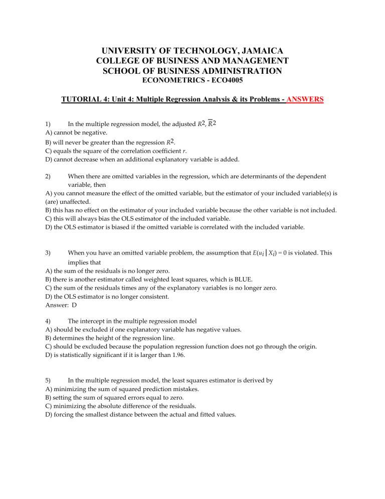
UNIVERSITY OF TECHNOLOGY, JAMAICA
COLLEGE OF BUSINESS AND MANAGEMENT
SCHOOL OF BUSINESS ADMINISTRATION
ECONOMETRICS - ECO4005
TUTORIAL 4: Unit 4: Multiple Regression Analysis & its Problems - ANSWERS
1)
In the multiple regression model, the adjusted R2,
A) cannot be negative.
B) will never be greater than the regression R2.
2
C) equals the square of the correlation coefficient r.
D) cannot decrease when an additional explanatory variable is added.
2)
When there are omitted variables in the regression, which are determinants of the dependent
variable, then
A) you cannot measure the effect of the omitted variable, but the estimator of your included variable(s) is
(are) unaffected.
B) this has no effect on the estimator of your included variable because the other variable is not included.
C) this will always bias the OLS estimator of the included variable.
D) the OLS estimator is biased if the omitted variable is correlated with the included variable.
3)
When you have an omitted variable problem, the assumption that E(ui Xi) = 0 is violated. This
implies that
A) the sum of the residuals is no longer zero.
B) there is another estimator called weighted least squares, which is BLUE.
C) the sum of the residuals times any of the explanatory variables is no longer zero.
D) the OLS estimator is no longer consistent.
Answer: D
4)
The intercept in the multiple regression model
A) should be excluded if one explanatory variable has negative values.
B) determines the height of the regression line.
C) should be excluded because the population regression function does not go through the origin.
D) is statistically significant if it is larger than 1.96.
5)
In the multiple regression model, the least squares estimator is derived by
A) minimizing the sum of squared prediction mistakes.
B) setting the sum of squared errors equal to zero.
C) minimizing the absolute difference of the residuals.
D) forcing the smallest distance between the actual and fitted values.
6)
The OLS residuals in the multiple regression model
A) cannot be calculated because there is more than one explanatory variable.
B) can be calculated by subtracting the fitted values from the actual values.
C) are zero because the predicted values are another name for forecasted values.
D) are typically the same as the population regression function errors.
7)
The population multiple regression model when there are two regressors, X1i and X2i can be
written as follows, with the exception of:
A) Yi = β0 + β1X1i + β2X2i + ui, i = 1,..., n
B) Yi = β0X0i + β1X1i + β2X2i + ui, X0i = 1, i = 1,..., n
2
C) Yi =

j 0
j
Xji + ui, i = 1,..., n
D) Yi = β0 + β1X1i + β2X2i + ... + βkXki + ui, i = 1,..., n
8)
In the multiple regression model, the SER is given by
1 n
 uˆi
n  2 i 1
n
1
B)
 ui
n  k  2 i 1
n
1
uˆi
C)

n  k  2 i 1
n
1
uˆi2
D)

n  k  2 i 1
A)
9)
In multiple regression, the R2 increases whenever a regressor is
A) added unless the coefficient on the added regressor is exactly zero.
B) added.
C) added unless there is heterosckedasticity.
D) greater than 1.96 in absolute value.
10)
The adjusted R2, or
, is given by
n  2 SSR
n  k  1 TSS
n  2 ESS
B) 1 
n  k  1 TSS
n  1 SSR
C) 1 
n  k  1 TSS
ESS
D)
TSS
A) 1 
11)
Consider the multiple regression model with two regressors X1 and X2, where both variables are
determinants of the dependent variable. When omitting X2 from the regression, then there will be
omitted variable bias for
A) if X1 and X2 are correlated
B) always
C) if X2 is measured in percentages
D) if X2 is a dummy variable
12)
The dummy variable trap is an example of
A) imperfect multicollinearity
B) something that is of theoretical interest only
C) perfect multicollinearity
D) something that does not happen to university or college students
QUESTION 13
Based on the data collected from 30 shops island-wide by the producers of a new brand of
vegetable loaf as at December 2010, the regression analysis was run which produced the
summary output below:
SUMMARY OUTPUT
Regression Statistics
Multiple R
0.952413257
R Square
0.907091012
Adjusted R
Square
0.675425058
Standard Error
1.767131177
Observations
30
ANOVA
Df
4
25
29
SS
135.9587
46.84129
182.8
Coefficients
-4,650.0001
-20.0005248
30.0001546
6.95000038
0.3000075
Standard
Error
2.002465
19.50003
1.400000
0.080001
0.220010
Regression
Residual
Total
Intercept
X Variable 1
X Variable 2
X Variable 3
X Variable 4
MS
33.98968
3.122753
F
5.780000
Significance
F
0.000241546
t Stat
P-value
1.07E-07
0.002192
0.671582
0.009752
0.237381
Lower 95%
20.4256009
-0.1340466
-0.2092916
-0.12816526
-0.02444292
Given:
Q = Quantity sold per month
X1 
P(in cents) = Price of the product = 900
X2  Py (in cents) = Price of leading competitor’s product = 850
X3  I (in dollars) = per capita income of the persons in the area in which the
shops are located = 16,500.
X4  E (in dollars) = Monthly advertising expenditure = 10,000
Using the information above,
a)
Develop the linear regression model for the Quantity of Vegetable Loaves demand
per month.
b)
What is the quality of the model (estimator) developed?
c)
What is the relationship and the strength of the relationship between
Demand for the Vegetable Loaves and the Independent Variables as a
group?
d)
Compute the t-statistics for each variable and state whether it is statistically
significant at the 5% level.
e)
Forecast the Demand for Vegetable Loaves using the model developed in
part a), based on the given information.
QUESTION 14
a) Using the data below, develop a multi-regression model for the demand
for soft drink using excel.
b) What is the quality of the estimator?
c) What Is the relationship and the strength of the relationship between the
dependent and independent variables?
d) Use the model to forecast the demand for soft drinks based on the values given.
Given the data below, gathered from 20 outlets in Kingston by the producers of a new Soft drink
as at December 2015.
Q
10
12
13
14
9
8
4
3
15
12
13
14
12
10
10
P
100
100
90
95
110
125
125
150
80
80
90
100
100
110
125
I
14
16
8
7
11
5
12
10
18
12
6
5
12
10
14
E
100
95
110
90
100
100
125
150
100
90
80
75
100
125
130
B
4
3
2
8
7
9
12
15
8
7
13
10
9
25
39
12
11
12
10
8
110
150
100
150
150
15
16
12
12
10
80
90
95
100
90
44
61
63
30
40
Given:
Q = Quantity (‘000) sold per month
P(in cents) = Price of the product = 70
I (in dollars) = per capita income of the persons in the area in which the
outlets are located = 6,500.
E (in dollars) = Monthly advertising expenditure = 100,000
B = Number of pizzas sold (per month in the area in which the
outlets are located.= 8,000.
15)
The cost of attending your college has once again gone up. Although you have been told that
education is investment in human capital, which carries a return of roughly 10% a year, you (and your
parents) are not pleased. One of the administrators at your university/college does not make the situation
better by telling you that you pay more because the reputation of your institution is better than that of
others. To investigate this hypothesis, you collect data randomly for 100 national universities and liberal
arts colleges from the 2000-2001 U.S. News and World Report annual rankings. Next you perform the
following regression
= 7,311.17 + 3,985.20 × Reputation – 0.20 × Size + 8,406.79 × Dpriv – 416.38 × Dlibart – 2,376.51 ×
Dreligion
R2=0.72, SER = 3,773.35
where Cost is Tuition, Fees, Room and Board in dollars, Reputation is the index used in U.S. News and
World Report (based on a survey of university presidents and chief academic officers), which ranges from
1 ("marginal") to 5 ("distinguished"), Size is the number of undergraduate students, and Dpriv, Dlibart,
and Dreligion are binary variables indicating whether the institution is private, a liberal arts college, and
has a religious affiliation.
(a) Interpret the results. Do the coefficients have the expected sign?
(b) What is the forecasted cost for a liberal arts college, which has no religious affiliation, a size of 1,500
students and a reputation level of 4.5? (All liberal arts colleges are private.)
(c) To save money, you are willing to switch from a private university to a public university, which has a
ranking of 0.5 less and 10,000 more students. What is the effect on your cost? Is it substantial?
(d) Eliminating the Size and Dlibart variables from your regression, the estimation regression becomes
= 5,450.35 + 3,538.84 × Reputation + 10,935.70 × Dpriv – 2,783.31 × Dreligion;
=0.72, SER = 3,792.68
Why do you think that the effect of attending a private institution has increased now?
(e) What can you say about causation in the above relationship? Is it possible that Cost affects Reputation
rather than the other way around?
16)
In the multiple regression model with two explanatory variables
Yi   0  1 X 1i   2 X 2i  ui
the OLS estimators for the three parameters are as follows (small letters refer to deviations from means as
in zi = Zi – Z ):
ˆ0  Y  ˆ1 X 1  ˆ2 X 2
n
n
n
n
 yi x1i  x22i   yi x2i  x1i x2i
ˆ1 
i 1
i 1
i 1
i 1


x12i  x22i    x1i x2i 

i 1
i 1
 i 1

n
n
n
ˆ2 
n
n
n
2
n
 y x x  y x x
i 1
i 2i
i 1
2
1i
i 1i
i 1
i 1
 n

x  x    x1i x2i 

i 1
i 1
 i 1

n
n
2
1i
x
1i 2 i
2
2
2i
You have collected data for 104 countries of the world from the Penn World Tables and want to estimate
the effect of the population growth rate ( X 1i ) and the saving rate ( X 2i ) (average investment share of
GDP from 1980 to 1990) on GDP per worker (relative to the U.S.) in 1990. The various sums needed to
n
calculate the OLS estimates are given below:
 Yi = 33.33;
i 1
n
y
i 1
2
i
n
= 8.3103;
n
yx
i 1
i 1i
x
i 1
2
1i
y x
i 1
i 2i
 X1i = 2.025;
i 1
n
X
i 1
2i
= 17.313
n
= .0122;
n
= -0.2304;
n
x
i 1
2
2i
= 0.6422
n
= 1.5676;
x
i 1
x = -0.0520
1i 2 i
(a) What are your expected signs for the regression coefficient? Calculate the coefficients and see if their
signs correspond to your intuition.
(b) Find the regression , and interpret it. What other factors can you think of that might have an
influence on productivity?
===========================================================