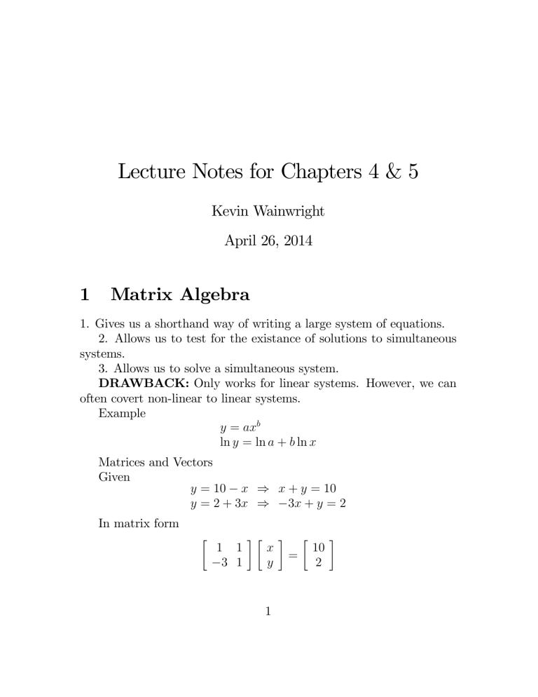
Lecture Notes for Chapters 4 & 5
Kevin Wainwright
April 26, 2014
1
Matrix Algebra
1. Gives us a shorthand way of writing a large system of equations.
2. Allows us to test for the existance of solutions to simultaneous
systems.
3. Allows us to solve a simultaneous system.
DRAWBACK: Only works for linear systems. However, we can
often covert non-linear to linear systems.
Example
y = axb
ln y = ln a + b ln x
Matrices and Vectors
Given
y = 10 x ) x + y = 10
y = 2 + 3x ) 3x + y = 2
In matrix form
1 1
3 1
x
y
1
=
10
2
Matrix of Coe¢ cients Vector of Unknows Vector of Constants
In general
a11 x1 + a12 x2 + : : : + a1n xn = d1
a21 x1 + a22 x2 + : : : + a2n xn = d2
::::::::::::::::::::::::::::::
am1 x1 + am2 x2 + : : : + amn xn = dm
n-unknowns (x1; x2; : : : xn )
Matrix form
2
a11
6 a21
6 .
4 ..
am1
Matrix shorthand
a12
a22
:::
am2
32
: : : a1n
6
: : : a2n 7
6
. . . ... 7
54
: : : amn
3 2
d1
x1
6 d2
x2 7
6 .
=
.. 7
. 5 4 ..
dm
xn
3
7
7
5
Ax = d
Where:
A= coe¢ cient martrix or an array
x= vector of unknowns or an array
d= vector of constants or an array
Subscript notation
aij
is the coe¢ cient found in the i-th row (i=1,. . . ,m) and the j-th
column (j=1,. . . ,n)
2
1.1
Vectors as special matrices
The number of rows and the number of columns de…ne the DIMENSION of a matrix.
A is m rows and n is columns or ”mxn.”
A matrix containing 1 column is called a ”column VECTOR”
x is a n 1 column vector
d is a m 1 column vector
If x were arranged in a horizontal array we would have a row vector.
Row vectors are denoted by a prime
x0 = [x1 ; x2 ; : : : ; xn ]
A 1 1 vector is known as a scalar.
x = [4] is a scalar
Matrix Operators
If we have two matrices, A and B, then
A = B if f
aij = bij
Addition and Subtraction of Matrices
Suppose A is an m n matrix and B is a p q matrix then A and
B is possible only if m=p and n=q. Matrices must have the same
dimensions.
a11 a12
a21 a22
+
b11 b12
b21 b22
=
(a11 + b11 ) (a12 + b12 )
(a21 + b21 ) (a22 + b22 )
c11 c12
c21 c22
=
Subtraction is identical to addition
9 4
3 1
7 2
1 6
=
(9
(3
7) (4
1) (1
3
2)
6)
=
2
2
2
5
Scalar Multiplication
Suppose we want to multiply a matrix by a scalar
k
1
A
m
1
We multiply every element in A by
2
ka11 ka12
6 ka21 ka22
kA = 6
4 ...
kam1 kam2
Example
n
the scalar k
3
: : : ka1n
: : : ka2n 7
7
5
: : : kamn
6 2
4 5
Let k=[3] and A=
then kA=
kA =
3
3
6 3
4 3
2
5
=
18 6
12 15
Multiplication of Matrices
To multiply two matrices, A and B, together it must be true that
for
A
B =
C
m n
n q
m q
That A must have the same number of columns (n) as B has rows
(n).
The product matrix, C, will have the same number of rows as A
and the same number of columns as B.
Example
A
B
(1 3)
1row
3cols
(3 4)
3rows
4cols
4
=
C
(1 4)
1row
4cols
In general
A
(3
B
2)
(2
C
5)
(5
D
4)
(4
=
1)
E
(3
1)
To multiply two matrices:
(1) Multiply each element in a given row by each element in a given
column
(2) Sum up their products
Example 1
b11 b12
b21 b22
a11 a12
a21 a22
Where:
c11 =a11 b11 + a12 b21
c12 =a11 b12 + a12 b22
c21 =a21 b11 + a22 b21
c22 =a21 b12 + a22 b22
Example 2
3 2
1 2
3 4
=
(sum
(sum
(sum
(sum
(3
of
of
of
of
row
row
row
row
1
1
2
2
1) +(2
=
times
times
times
times
3) (3
c11 c12
c21 c22
column
column
column
column
1)
2)
1)
2)
2) +(2
4)
=
9 14
Example 3
2
3
2
3 2 1 415=
4
(3
2) + (2
1) + (1
12 is the inner product of two vectors.
Suppose
x=
x1
x2
then x0 =
5
x1 x2
4)
= [12]
therefore
x0 x =
x1
x2
x1 x2
= x21 + x22
However
xx0 = 2 by 2 matrix
x1
x2
Example 4
x1 x2
=
2
3
1 3
A=42 85
4 0
5
9
b=
2
Example
x21 x1 x2
x2 x1 x22
(1
Ab = 4 (2
(4
5) + (3
5) + (8
5) + (0
3
3 2
32
9)
9) 5 = 4 82 5
20
9)
Ax = d
A
2 d 3
3 2 x3
6 3 1
22
x1
41 4
5
4
5
4
2
x2 =
12 5
4 1 5
x3
10
(3 3)
(3 1) (3 1)
2
6
This produces
6x1 + 3x2 + x3 = 22
x1 + 4x2 2x3 = 12
4x1 x2 + 5x3 = 10
1.1.1
National Income Model
y = c + I0 + G0
C = a + bY
Arrange as
y
C = I0 + G0
bY + C = a
Matrix form
A
1
b
1.1.2
1
1
x
Y
C
=
=d
Io + Go
a
Division in Matrix Algebra
In ordinary algebra
a
=c
b
is well de…ned i¤ b6= 0.
Now 1b can be rewritten as b 1 ; therefore ab
But in matrix algebra
A
=C
B
is not de…ned. However,
AB
1
7
=C
1
= c; also b 1 a = c:
is well de…ned. BUT
1
AB
B
1
6= B 1 A
is called the inverse of B
B
1
6=
1
B
In some ways B 1 has the same properties as b
it di¤ers. We will explore these di¤erences later.
1.2
1
but in other ways
Commutative, Associative, and Distributive
Laws
From Highschool algebra we know commutative law of addition,
a+b=b+a
commutative law of multiplication,
ab = ba
Associative law of addition,
(a + b) + c = a + (b + c)
associative law of multiplication,
(ab)c = a(bc)
Distributive law
a(b + c) = ab + ac
In matrix algebra most, but not all, of these laws are true.
8
1.2.1
I) Communicative Law of Addition
A+B =B+A
Since we are adding individual elements and aij + bij = bij + aij for
all i and j.
1.2.2
II) Similarly Associative Law of Addition
A + (B + C) = (A + B) + C
for the same reasons.
1.2.3
III) Matrix Multiplication
Matrix multiplication in not communtative
IB 6= BA
Example 1
Let A be 2 3 and B be 3 2
A
(2
B
3)
(3
Example 2
1 2
Let A=
3 4
AB =
=
2)
C
(2
and B=
whereas
2)
0
6
B
A
(3
2)
1) + (2
1) + (4
7)
7)
(2
=
3)
1
7
(1 10) + (2 6) (1
(3 0) + (4 6) (3
9
=
12 13
24 25
C
(3
3)
But
BA =
(0)(1) (1)(3) (0)(2) (1)(4)
(6)(1) + (7)(3) (6)(2) + (7)(4)
=
3 4
27 40
Therefore, we realize the distinction of post multiply and pre multiply. In the case
AB = C
B is pre multiplied by A, A is post multiplied by B.
1.2.4
IV) Associative Law
Matrix multiplication is associative
(AB)C = A(BC) = ABC
as long as their dimensions conform to our earlier rules of multiplication.
A
B
C
(m n)
(n p)
(p q)
1.2.5
V) Distributive Law
Matrix multiplication is distributive
A(B + C) = AB + AC Pre multiplication
(B + C)A = BA + CA Post multiplication
10
1.3
1.3.1
Identity Matrices and Null Matrices
Identity matrix:
is a square matrix with ones on its principal diagonals and zeros everywhere else.
3
2
1 0 ::: n
3
2
1 0 0
.. 7
6
. 7
1 0
60 1
5
4
In = 6 .
I2 =
I3 = 0 1 0
.
..
.. 0 7
0 1
5
4
0 0 1
0 ::: 0 1
Identity Matrix in scalar algebra we know
1
a=a
1=a
In matrix algebra the identity matrix plays the same role
IA = AI = A
Example 1
1 3
Let A=
2 4
IA =
1 0
0 1
1 3
2 4
=
(1
(0
1) + (0
1) + (1
2) (1
2) (0
3) + (0
3) + (1
4)
4)
Example 2
1 2 3
Let A=
2 0 3
IA =
1 0
0 1
1 2 3
2 0 3
=
11
1 2 3
2 0 3
= A fI2 Caseg
=
1 3
2 4
AI =
1 2 3
2 0 3
Furthermore,
AIB
(m n)(n
1.3.2
2
3
1 0 0
40 1 05=
0 0 1
1 2 3
2 0 3
= A fI3 Caseg
= (AI)B = A(IB) =
p)
(m
AB
n)(n
p)
Null Matrices
A null matrix is simply a matrix where all elements equal zero.
0 0
0 0
(2 2)
0=
0=
0 0 0
0 0 0
(2 3)
The rules of scalar algebra apply to matrix algebra in this case.
Example
a + 0 = a ) fscalarg
A+0=
A
0=
a11 a12
a21 a22
0 0
0 0
+
a11 a12 a13
a21 a22 a23
12
=A
2
3
0
=405=
0
fmatrixg
0
0
=0
1.4
Idiosyncracies of matrix algebra
1) We know AB6=BA
2)ab=0 implies a or b=0
In matrix
AB =
1.4.1
2 4
1 2
2
1
4
2
=
0 0
0 0
Transposes and Inverses
1)Transpose: is when the rows and columns are interchanged.
Transpose of A=A’or AT
Example
3
3 8 9
and B=
If A=
1
1 0 4
2
3
3 1
3 4
A’=4 8 0 5 and B’=
1 7
9 4
Symmetrix Matrix
2
3
2
1 0 4
1
If A=4 0 3 7 5 then A’=4 0
4 7 2
4
A is a symmetric matrix.
4
7
3
0 4
3 75
7 2
Properties of Transposes
1) (A0)0 = A
2) (A + B)0 = A0 + B0
3) (AB)0 = B0A0
Inverses and their Properties
13
In scalar algebra if
ax = b
then
x=
b
or ba
a
1
In matrix algebra, if
Ax = d
then
x = A 1d
where A
1
is the inverse of A.
Properties of Inverses
1) Not all matrices have inverses
non-singular: if there is an inverse
singular: if there is no inverse
2) A matrix must be square in order to have an inverse. (Necessary
but not si¢ cient)
3) In scalar algebra aa = 1; in matrix algebra AA 1 = A 1 A = I
4) If an inverse exists then it must be unique.
Example
3 1
Let A=
0 2
and A
1
=
1
3
1
2
0
2 1
by factoring
0 3
Post Multiplication
A
1
=
1
6
AA
1
=
3 1
0 2
2
0
1
3
1
6
1
6
is a scalar
1
=
6
14
6 0
0 6
1
=
6
1 0
0 1
Pre Multiplication
A 1A =
1
6
2
0
1
3
3 1
0 2
=
1
6
6 0
0 6
1 0
0 1
=
Further properties
If A and B are square and non-singular then:
1) (A 1 ) 1 = A
2) (AB) 1 = B 1 A 1
3) (A0) 1 = (A 1 )1
Solving a linear system
Suppose
A
(3
then
x
3) (3
=
1)
d
(3
1)
A 1
A
x
= A 1
d
(3 3) (3 3) (3 1)
(3 3) (3 1)
I
(3
x
3) (3
=
1)
A 1
d
(3 3) (3 1)
x = A 1d
Example
2
6
A=41
4
then
3
4
1
2
3
2
Ax
3 =d 2
3
22
d = 4 12 5
10
1
x1
2 5 x = 4 x2 5
5
x3
3
2
x1
18
1
4 13
4 x2 5 =
52
x3
17
16
26
18
1
18
1 4
13
=
52
17
32
3 2 3
10
22
2
13 5 4 12 5 = 4 3 5
21
10
1
x1 = 2 x2 = 3 x3 = 1
15
A
2
16
26
18
3
10
13 5
21
1.5
Linear Dependence and Determinants
Suppose we have the following
1: x1 + 2x2 = 1
2: 2x1 + 4x2 = 2
where equation two is twice equation one. Therefore, there is no
solution for x1 ; x2 :
In matrix form:
Ax = d
"
A
1 2
2 4
#"
x
x1
x2
#
=
"
d
1
2
#
The determinant of the coe¢ cient matrix is
jAj = (1)(4)
(2)(2) = 0
a determinant of zero tells us that the equations are linearly dependent. Sometimes called a ”vanishing determinant.”
In general, the determinant of a square matrix, A is written as jAj
or detA.
For two by two case
jAj =
a11 a12
= a11 a22
a21 a22
where k is unique
any k6= 0 implies linear independence
Example 1
16
a12 a21 = k
A=
3 2
1 5
jAj = (3
5)
(1
fNon-singularg
2) = 13
Example 2
2 6
B=
8 24
jBj = (2
Three by three
2
a1
4
Given A= b1
c1
then
24)
(6
8) = 0
case 3
a2 a3
b2 b3 5
c2 c3
jAj = (a1 b2 c3 ) + (a2 b3 c1 ) + (b1 c2 a3 )
Cross-diagonals
fSingularg
(a3 b2 c1 )
(a2 b1 c3 )
(b3 c2 a1 )
3
a1 a2 a3
4 b1 b2 b3 5
c1 c2 c3
2
Use viso to display cross diagonals
Multiple along the diagonals and add up their products
)The product along the BLUE lines are given a positive sign
)The product of the RED lines are negative.
17
1.6
Using Laplace expansion
) The cross diagonal method does not work for matrices greater than
three by three
) Laplace expansion evaluates the determinant of a matrix, A, by
means of subdeterminants of A.
Subdeterminants
or Minors
3
2
a1 a2 a3
Given A=4 b1 b2 b3 5
c1 c2 c3
By deleting the …rst row and …rst column, we get
b2 b3
c2 c3
jM11 j =
The determinant of this matrix is the minor element a1 .
jMij j
is the subdeterminant from deleting the i-th row and the
j-th column.
3
2
a1 a2 a3
Given A=4 b1 b2 b3 5
c1 c2 c3
then
a12 a13
a12 a13
M21
M31
a32 a33
a22 a23
1.6.1
Cofactors
A cofactor is a minor with a speci…c algebraic sign.
Cij = ( 1)i+j jMij j
therefore
C11 = ( 1)2 jM11 j = jM11 j
C21 = ( 1)3 jM21 j = jM21 j
18
The determinant by Laplace
2
a11
A = 4 a21
a31
Expanding down the …rst column
3
a12 a13
a22 a23 5
a32 a33
jAj = a11 jC11 j + a21 jC21 j + a31 jC31 j =
jAj = a11
a22 a23
a32 a33
a21
3
X
i=1
ai1 jCi1 j
a12 a13
a a
+ a31 12 13
a22 a23
a32 a33
Note: minus sign ( 1)(1+2)
jAj = a11 [a22 a33
a23 a32 ]
a21 [a12 a33
a13 a32 ] + a31 [a12 a23
a13 a22 ]
Laplace expansion can be used to expand along any row or any
column.
Example: Third row
jAj = a31
a12 a13
a22 a23
a32
a a
a11 a13
+ a33 11 12
a21 a22
a21 a23
Example
2
3
8 1 3
A=44 0 15
6 0 3
(1)Expand the …rst column
jAj = 8
0 1
0 3
4
19
1 3
1 3
+6
0 3
0 1
jAj = (8
0)
jAj =
8 3
4 1
+0
6 3
6 3
(4
3) + (6
1) =
6
(2) Expand the second column
1
jAj = ( 1
6) + (0)
0
(0) =
8 3
4 1
6
Suggestion: Try to choose an easy row or column to expand. (i.e. the
ones with zero’s in it.)
1.7
Matrix Inversion
Given an n n matrix, A, the inverse of A is
A
1
=
1
jAj
AdjA
where AdjA is the adjoint matrix of A. AdjA is the transpose of
matrix A’s cofactor matrix. It is also the adjoint, which is an n n
matrix
Cofactor Matrix (denoted C)
The cofactor matrix of A is a matrix who’s elements are the cofactors of the elements of A
If A =
a11 a12
a21 a22
jC11 j jC12 j
jC21 j jC22 j
then C =
Example
Let A=
3 2
1 0
) jAj=-2
20
=
a22
a12
a21
a11
Step 1: Find the cofactor matrix
C=
jC11 j jC12 j
jC21 j jC22 j
=
0
2
1
3
Step 2: Transpose the cofactor matrix
C T = AdjA =
0
1
2
3
1
jAj
Step 3: Multiply all the elements of AdjA by
A
1
=
1
jAj
Step 4: Check by AA
0
3 2
1
1 0
2
1 0
=
0 1
1.8
1
2
AdjA =
1
3
2
1
0
1
2
3
=
0
1
1
2
3
2
=I
=
(3)(0) + (2)( 12 ) (3)(1) + (2)(
(1)(0) + (0)( 12 ) (1)(1) + (0)(
Cramer’s Rule
Suppose:
Equation 1 a1 x1 + a2 x2 = d1
Equation 2 b1 x1 + b2 x2 = d2
or
to …nd A
A
a1 a2
b1 b2
x
x1
x2
21
=
=
d
d1
d2
3
2)
3
2)
1
where
a2 b1 6= 0
A = a1 b 2
Solve for x1 by substitution
From equation 1
x2 =
d1
a1 x1
a2
and equation 2
x2 =
therefore:
d1
d2
a1 x 1
a2
b1 x1
b2
=
d2
b1 x1
b2
Cross multiply
d1 b2
a1 b2 x1 = d2 a2
b 1 a2 x 1
Collect terms
d1 b2
d2 a2 = (a1 b2 b1 a2 )x1
d1 b2 d2 a2
x1 =
a1 b2 b1 a2
The denominator is the determinant of jAj and the numerator is the
same as the denominator except d1 d2 replaces a1 b1 :
Cramer’s Rule
x1 =
d1
d2
a1
b1
a2
b2
a2
b2
=
d1 b2
a1 b2
d 2 a2
b 1 a2
Where the d vector replaces column 1 in the A matrix
22
To …nd x2 replace column 2 with the d vector
x2 =
a1
b1
a1
b1
d1
d2
a2
b2
a1 d2
a1 b2
=
d1 b1
b 1 a2
Generally: to …nd xi ;replace column i with vector d; …nd the determinant.
xi = the ratio of two determinants
ij
xi = jA
jAj
1.8.1
Example: The Market Model
Equation 1 Qd = 10
P Or Q + P = 10
Equation 2 Qs = P
2 Or
Matrix form
Find Qe
A
1 1
1 1
x
Q
P
jAj = (1)(1)
Qe =
Find Pe
Pe =
10 1
2 1
2
1 10
1 2
2
Q+P =2
=
d
10
2
=
( 1)(1) = 2
=
=
23
10
2
2
2
=4
( 10)
=6
2
Substitute P and Q into either equation 1 or equation 2 to verify
Qd = 10 P
10 6 = 4
1.8.2
Example: National Income Model
Y = C + I0 + G0 Or Y
C = a + bY Or
C = I0 + G0
bY + c = a
In matrix form
1
b
Solve for Y e
Ye =
1
1
Y
C
I0 + G0
1
a
1
1
1
b 1
I0 + G0
a
=
=
I0 + G0 + a
1 b
Solve for C e
Ce =
1 I0 + G0
b
a
1
1
b 1
=
a + b(I0 + G0 )
1 b
Numeric example:
Let C = 100 + 0:75Y; I = 150 and G = 250. Then the model is
Y
Y
C = I +G
C = 400
24
and
0:75Y
C = 100 + 0:75Y
C = 100
In Matrix form
1
0:75
Solve for Y e
Ye =
1
1
Y
C
400 1
100 1
1
1
0:75 1
=
=
400
100
500
= 2000
0:25
Solve for C e
Ce =
1
400
0:75 100
1
1
0:75 1
=
100 + 0:75(400)
= 1600
0:25
25