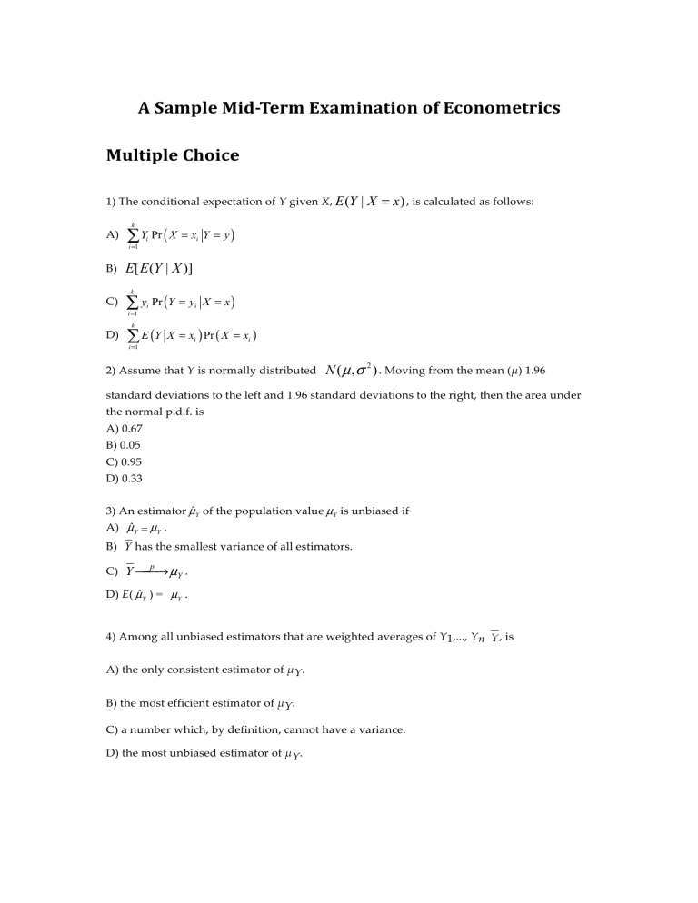
A Sample Mid-Term Examination of Econometrics
Multiple Choice
1) The conditional expectation of Y given X, E (Y
A)
k
∑ Y Pr ( X = x
i =1
i
Y = y)
i
X = x)
i
B)
E[ E (Y | X )]
C)
∑ y Pr (Y = y
k
i =1
D)
i
k
∑ E (Y
i =1
| X = x) , is calculated as follows:
X = xi ) Pr ( X = xi )
2) Assume that Y is normally distributed
N ( µ , σ 2 ) . Moving from the mean (µ) 1.96
standard deviations to the left and 1.96 standard deviations to the right, then the area under
the normal p.d.f. is
A) 0.67
B) 0.05
C) 0.95
D) 0.33
3) An estimator µˆY of the population value µY is unbiased if
A) µˆY = µY .
B) Y has the smallest variance of all estimators.
C) Y ⎯
⎯→ µY .
p
D) E( µˆY ) = µY .
4) Among all unbiased estimators that are weighted averages of Y1,..., Yn
A) the only consistent estimator of µY.
B) the most efficient estimator of µY.
C) a number which, by definition, cannot have a variance.
D) the most unbiased estimator of µY.
, is
5) Assume that you have 125 observations on the height (H) and weight (W) of your peers in
college.
Let
= 68,
= 3.5,
= 29. The sample correlation coefficient is
A) 1.22
B) 0.50
C) 0.67
D) Cannot be computed since males and females have not been separated out.
6) When the estimated slope coefficient in the simple regression model,
1, is zero, then
A) R2 =
.
2
B) 0 < R < 1.
C) R2 = 0.
D) R2 > (SSR/TSS).
7) The reason why estimators have a sampling distribution is that
A) economics is not a precise science.
B) individuals respond differently to incentives.
C) in real life you typically get to sample many times.
D) the values of the explanatory variable and the error term differ across samples.
8) The variance of Yi is given by
A)
+
var(Xi) + var(ui).
B) the variance of ui.
C)
var(Xi) + var(ui).
D) the variance of the residuals.
9) To obtain the slope estimator using the least squares principle, you divide the
A) sample variance of X by the sample variance of Y.
B) sample covariance of X and Y
C) sample covariance of
D) sample variance of
by the sample variance of Y.
X and Y by the sample variance of X.
X by the sample covariance of
X and Y.
10) Changing the units of measurement, e.g. measuring testscores in 100s, will do all of the
following EXCEPT for changing the
A) residuals
B) numerical value of the slope estimate
C) interpretation of the effect that a change in X has on the change in Y
D) numerical value of the intercept
11) Heteroskedasticity means that
A) homogeneity cannot be assumed automatically for the model.
B) the variance of the error term is not constant.
C) the observed units have different preferences.
D) agents are not all rational.
12) The t-statistic is calculated by dividing
A) the OLS estimator by its standard error.
B) the slope by the standard deviation of the explanatory variable.
C) the estimator minus its hypothesized value by the standard error of the estimator.
D) the slope by 1.96.
13) The 95% confidence interval for β1 in large samples is the interval
A) (β1 - 1.96SE(β1), β1 + 1.96SE(β1)).
B) ( 1 - 1.645SE( 1),
C) ( 1 - 1.96SE( 1),
D) ( 1 - 1.96,
1 + 1.645SE( 1)).
1 + 1.96SE( 1)).
1 + 1.96).
14) Consider the estimated equation from your textbook
=698.9 - 2.28 STR, R2 = 0.051, SER = 18.6
(10.4) (0.52)
The t-statistic for the slope is approximately
A) 4.38
B) 67.20
C) 0.52
D) 1.76
15) Using 143 observations, assume that you had estimated a simple regression function and
that your estimate for the slope was 0.04, with a standard error of 0.01. You want to test
whether or not the estimate is statistically significant. Which of the following possible
decisions is the only correct one:
A) you decide that the coefficient is small and hence most likely is zero in the population
B) the slope is statistically significant since it is four standard errors away from zero
C) the response of Y given a change in X must be economically important since it is
statistically significant
D) since the slope is very small, so must be the regression R2.
16) Under imperfect multicollinearity
A) the OLS estimator cannot be computed.
B) two or more of the regressors are highly correlated.
C) the OLS estimator is biased even in samples of n > 100.
D) the error terms are highly, but not perfectly, correlated.
17) When you have an omitted variable problem, the assumption that E(ui Xi) = 0 is
violated. This implies that
A) the sum of the residuals is no longer zero.
B) there is another estimator called weighted least squares, which is BLUE.
C) the sum of the residuals times any of the explanatory variables is no longer zero.
D) the OLS estimator is no longer consistent.
18) In the multiple regression model Yi = β0 + β1X1i+ β2 X2i + ... + βkXki + ui, i = 1,..., n, the
OLS estimators are obtained by minimizing the sum of
A) squared mistakes in
B) squared mistakes in
C) absolute mistakes in
D) squared mistakes in
n
∑ (Y − b
0
− b1 X 1i −
− bk X ki )
∑ (Y − b
0
− b1 X 1i −
− bk X ki − ui )
i =1
n
i =1
n
i
i
∑ (Y − b
− b1 X 1i −
∑ (Y − b
− b1 X i )
i
i =1
n
i =1
i
0
0
2
2
− bk X ki )
2
19) In the multiple regression model, the SER is given by
1 n
∑ uˆi
n − 2 i =1
n
1
B)
ui
∑
n − k − 2 i =1
n
1
C)
uˆi
∑
n − k − 2 i =1
n
1
D)
uˆi2
∑
n − k − 2 i =1
A)
20) Consider the following multiple regression models (a) to (d) below. DFemme = 1 if the
individual is a female, and is zero otherwise; DMale is a binary variable which takes on the
value one if the individual is male, and is zero otherwise; DMarried is a binary variable which
is unity for married individuals and is zero otherwise, and DSingle is (1-DMarried).
Regressing weekly earnings (Earn) on a set of explanatory variables, you will experience
perfect multicollinearity in the following cases unless:
A)
i=
+
DFemme +
Dmale +
B)
i=
+
DMarried +
DSingle +
C)
i=
+
DFemme +
X3i
X3i
X3i
D)
i=
DFemme +
Dmale +
DMarried +
DSingle +
X3i
Long Questions
1. The OLS formula for the slope coefficients in the multiple regression model become
increasingly more complicated, using the "sums" expressions, as you add more regressors.
For example, in the regression with a single explanatory variable, the formula is
∑( X
)(
n
i =1
− X Yi − X
i
∑( X
n
i =1
−X
i
)
)
2
Show that for a multiple regression model
Yi = β0 + β1 X1 + β2 X 2 + u2
the formula for the slope of the first explanatory variable is
n
βˆ1 =
n
n
n
∑ y x ∑ x −∑ y x ∑ x
i =1
i 1i
i =1
2
2i
i =1
i 2i
i =1
⎛ n
⎞
x ∑ x − ⎜ ∑ x1i x2i ⎟
∑
i =1
i =1
⎝ i =1
⎠
n
2
1i
n
x
1i 2 i
2
2
2i
(small letters refer to deviations from means as in zi = Zi − Z . Hint: use the FWL theorem to
reduce the model to a multiple regression model without an intercept. Then use the matrix
formula of β̂ for the reduced model.)
2 Sir Francis Galton, a cousin of James Darwin, examined the relationship between the height
of children and their parents towards the end of the 19th century. It is from this study that the
name "regression" originated. You decide to update his findings by collecting data from 110
college students, and estimate the following relationship:
= 19.6 + 0.73 × Midparh, R2 = 0.45, SER = 2.0
(7.2)
(0.10)
where Studenth is the height of students in inches, and Midparh is the average of the parental
heights. Values in parentheses are heteroskedasticity robust standard errors. (Following
Galton's methodology, both variables were adjusted so that the average female height was
equal to the average male height.)
(a) Test for the statistical significance of the slope coefficient.
(b) If children, on average, were expected to be of the same height as their parents, then this
would imply two hypotheses, one for the slope and one for the intercept.
(i) What should the null hypothesis be for the intercept? Calculate the relevant t-statistic and
carry out the hypothesis test at the 1% level.
(ii) What should the null hypothesis be for the slope? Calculate the relevant t-statistic and
carry out the hypothesis test at the 5% level.
(c) Can you reject the null hypothesis that the regression R2 is zero?
(d) Construct a 95% confidence interval for a one inch increase in the average of parental
height.
Answers
Multiple Choice
1) C
2) C
3) D
4) B
5) C
6) C
7) D
8) C
9) C
10) C
11) B
12) C
13) C
14) A
15) B
16) B
17) D
18) A
19) D
20) C
Long Questions
1. We will demonstrate this question in class.
2.
(a) H0 : β1 = 0, t=7.30, for H1 : β1 > 0, the critical value for a two-sided alternative is 1.645.
Hence we reject the null hypothesis
(b) H0 : β0 = 0, t=2.72, for H1 : β0 ≠ 0, the critical value for a two-sided alternative is 2.58.
Hence we reject the null hypothesis in (i). For the slope we have H0 : β1 = 1, t=-2.70, for H1 :
β1 ≠ 1, the critical value for a two-sided alternative is 1.96. Hence we reject the null hypothesis
in (ii).
(c) For the simple linear regression model, H0 : β1 = 0 implies that R2 = 0.
same test as in (a).
Hence it is the
(d) (0.73 – 1.96 × 0.10, 0.73 + 1.96 × 0.10) = (0.53, 0.93).