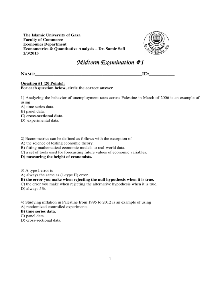
The Islamic University of Gaza
Faculty of Commerce
Economics Department
Econometrics & Quantitative Analysis – Dr. Samir Safi
2/3/2013
Midterm Examination #1
NAME:______________________________________________ID:___________
Question #1 (20 Points):
For each question below, circle the correct answer
1) Analyzing the behavior of unemployment rates across Palestine in March of 2006 is an example of
using
A) time series data.
B) panel data.
C) cross-sectional data.
D) experimental data.
2) Econometrics can be defined as follows with the exception of
A) the science of testing economic theory.
B) fitting mathematical economic models to real-world data.
C) a set of tools used for forecasting future values of economic variables.
D) measuring the height of economists.
3) A type I error is
A) always the same as (1-type II) error.
B) the error you make when rejecting the null hypothesis when it is true.
C) the error you make when rejecting the alternative hypothesis when it is true.
D) always 5%.
4) Studying inflation in Palestine from 1995 to 2012 is an example of using
A) randomized controlled experiments.
B) time series data.
C) panel data.
D) cross-sectional data.
1
5) The correlation coefficient
A) lies between zero and one.
B) is a measure of linear association.
C) is close to one if X causes Y.
D) takes on a high value if you have a strong nonlinear relationship.
6) Analyzing the effect of minimum wage changes on teenage employment across the 48 contiguous
U.S. states from 1990 to 2012 is an example of using
A) time series data.
B) panel data.
C) having a treatment group vs. a control group, since only teenagers receive minimum wages.
D) cross-sectional data.
7) Binary variables
A) are generally used to control for outliers in your sample.
B) can take on more than two values.
C) exclude certain individuals from your sample.
D) can take on only two values.
8) In the simple linear regression model, the regression slope
A) indicates by how many percent Y increases, given a one percent increase in X.
B) when multiplied with the explanatory variable will give you the predicted Y.
C) indicates by how many units Y increases, given a one unit increase in X.
D) represents the elasticity of Y on X.
9) The OLS estimator is derived by
A) connecting the Yi corresponding to the lowest Xi observation with the Yi corresponding to the
highest Xi observation.
B) making sure that the standard error of the regression equals the standard error of the slope estimator.
C) minimizing the sum of absolute residuals.
D) minimizing the sum of squared residuals.
10) The sample average of the OLS residuals is
A) some positive number since OLS uses squares.
B) zero.
C) unobservable since the population regression function is unknown.
D) dependent on whether the explanatory variable is mostly positive or negative.
11) The OLS residuals
A) can be calculated using the errors from the regression function.
B) can be calculated by subtracting the fitted values from the actual values.
C) are unknown since we do not know the population regression function.
2
D) should not be used in practice since they indicate that your regression does not run through all your
observations.
12) The regression R2 is a measure of
A) whether or not X causes Y.
B) the goodness of fit of your regression line.
C) whether or not ESS > TSS.
D) the square of the determinant of R.
13) Multiplying the dependent variable by 100 and the explanatory variable by 100,000 leaves the
A) OLS estimate of the slope the same.
B) OLS estimate of the intercept the same.
C) regression R2 the same.
D) variance of the OLS estimators the same.
14) Assume that you have collected a sample of observations from over 100 households and their
consumption and income patterns. Using these observations, you estimate the following regression Ci
= β0+β1Yi+ ui where C is consumption and Y is disposable income. The estimate of β1 will tell you
A)
∆Income
∆Consumption
B) The amount you need to consume to survive
C)
Income
Consumption
D)
∆Consumption
∆Income
15) The t-statistic is calculated by dividing
A) the OLS estimator by its standard error.
B) the slope by the standard deviation of the explanatory variable.
C) the estimator minus its hypothesized value by the standard error of the estimator.
D) the slope by 1.96.
16) The confidence interval for the sample regression function slope
A) can be used to conduct a test about a hypothesized population regression function slope.
B) can be used to compare the value of the slope relative to that of the intercept.
C) adds and subtracts 1.96 from the slope.
D) allows you to make statements about the economic importance of your estimate.
17) Finding a small value of the p-value (for example less than 5%)
A) indicates evidence in favor of the null hypothesis.
3
B) implies that the t-statistic is less than 1.96.
C) indicates evidence in against the null hypothesis.
D) will only happen roughly one in twenty samples.
18) One of the following steps is not required as a step to test for the null hypothesis:
A) compute the standard error of 1.
B) test for the errors to be normally distributed.
C) compute the t-statistic.
D) compute the p-value.
19) In the multiple regression model, the adjusted R2, 2
A) cannot be negative.
B) will never be greater than the regression R2.
C) equals the square of the correlation coefficient r.
D) cannot decrease when an additional explanatory variable is added.
20) When testing joint hypothesis, you should
A) use t-statistics for each hypothesis and reject the null hypothesis if all of the restrictions fail.
B) use the F-statistic and reject all of regression coefficients if p-value (Sig./Prob.) ≤ α .
C) use t-statistics for each hypothesis and reject the null hypothesis if p-value (Sig./Prob.) ≤ α .
D) use the F-statistics and reject at least one of the regression coefficient if p-value (Sig./Prob.)
≤α.
4
Question #2 (10 Points):
Consider the annual demand for fish. Ft, the average pounds of fish consumed per capita in year t, PFt,
the price index for fish in year t, PBt, the price index for beef in year t, and Ydt, the real per capita
disposable income in year t.
(a) (2 Points) Write the estimated regression equation of Ft on PFt , PBt and Ydt
(b) (2 Points) Test the significance for the estimated slope coefficient of Ydt at 0.05 level.
(c) (2 Points) Test for the overall significance of the estimated equation at 0.05 level.
(d) (2 Points) Interpret the 95% confidence interval for the estimated slope coefficient for PFt
(e) (2 Points) Interpret the adjusted coefficient of determination.
5
Eviews Output
Dependent Variable: F
95% CI
Variable
Coefficient
Std. Error
t-Statistic
Prob.
Low
High
C
PF
PB
YD
10.53269
0.025722
0.005440
0.000133
0.410714
0.027325
0.018661
0.000555
25.64481
0.941354
0.291496
0.240020
0.0000
0.3572
0.7735
0.8126
9.678562
-0.031103
-0.033368
-0.001021
11.38682
0.082547
0.044248
0.001288
R-squared
F-statistic
0.719687
17.97204
Adjusted R-squared
Prob(F-statistic)
6
0.679642
0.000005