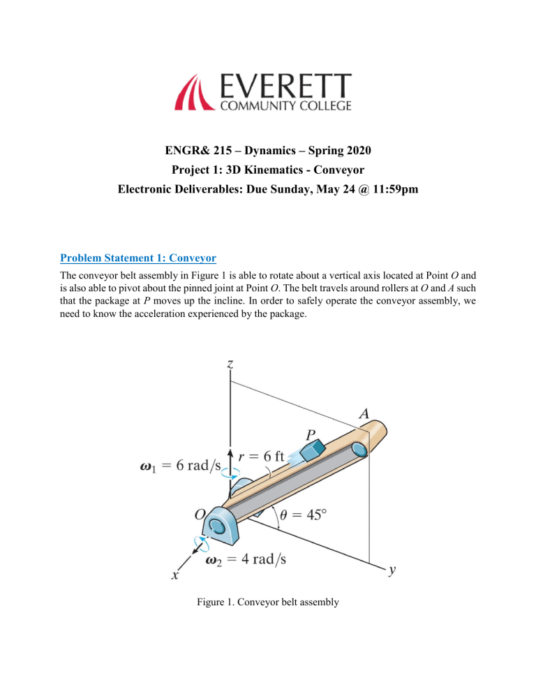
ENGR& 215 – Dynamics – Spring 2020
Project 1: 3D Kinematics - Conveyor
Electronic Deliverables: Due Sunday, May 24 @ 11:59pm
Problem Statement 1: Conveyor
The conveyor belt assembly in Figure 1 is able to rotate about a vertical axis located at Point O and
is also able to pivot about the pinned joint at Point O. The belt travels around rollers at O and A such
that the package at P moves up the incline. In order to safely operate the conveyor assembly, we
need to know the acceleration experienced by the package.
Figure 1. Conveyor belt assembly
Instructions for Calculations
All tasks are to be completed in groups!
1- By hand, calculate the magnitude of the velocity and acceleration of the package, using the
following information:
a) The angle marked theta (Figure 1) is 45⁰.
b) At this instant, the entire assembly rotates around a vertical axis located at Point O (in
the direction shown in Figure 1) with an angular velocity of 6 rad/s.
c) At this instant, the conveyor arm pivots about point O (in the direction shown in Figure
1) with an angular velocity of 4 rad/s.
d) At this instant, the belt is running at rate of 5 ft/s, which is increasing at a rate of 8 ft/s2.
2- Using MS Excel or MATLAB:
a) Determine how the acceleration of the package changes relative to the angular
acceleration of the assembly about the vertical axis (zero in Part 1). In your
calculations, keep all other variables constant, using the values given in Part 1. Vary
the angular acceleration of the assembly between 0 and 15 rad/s2.
b) Determine how the acceleration of the package changes relative to the angular
acceleration of the conveyor arm as it pivots (zero in Part 1). In your calculations, keep
all other variables constant, using the values given in Part 1. Vary the angular
acceleration of the conveyor arm between 0 and 15 rad/s2.
c) Determine how the acceleration of the package changes relative to the magnitude of
linear acceleration of the boom (given as 8 ft/s2 in Part 1). In your calculations, keep
all other variables constant, using the values given in Part 1. Vary the magnitude of the
linear acceleration between 0 and 30 ft/s2.
Note

Make sure to show these results graphically and discuss them in your presentation.

Make sure to plot enough data points to ensure that your curves are smooth.

Plot the results for Parts 2.a) and b) on the same graph, using the same axes, and compare
the results.