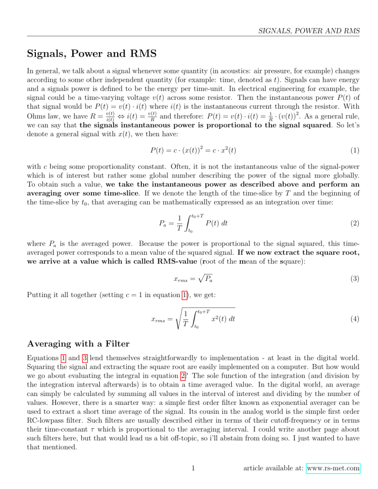
SIGNALS, POWER AND RMS
Signals, Power and RMS
In general, we talk about a signal whenever some quantity (in acoustics: air pressure, for example) changes
according to some other independent quantity (for example: time, denoted as t). Signals can have energy
and a signals power is defined to be the energy per time-unit. In electrical engineering for example, the
signal could be a time-varying voltage v(t) across some resistor. Then the instantaneous power P (t) of
that signal would be P (t) = v(t) · i(t) where i(t) is the instantaneous current through the resistor. With
⇔ i(t) = v(t)
and therefore: P (t) = v(t) · i(t) = R1 · (v(t))2 . As a general rule,
Ohms law, we have R = v(t)
i(t)
R
we can say that the signals instantaneous power is proportional to the signal squared. So let’s
denote a general signal with x(t), we then have:
P (t) = c · (x(t))2 = c · x2 (t)
(1)
with c being some proportionality constant. Often, it is not the instantaneous value of the signal-power
which is of interest but rather some global number describing the power of the signal more globally.
To obtain such a value, we take the instantaneous power as described above and perform an
averaging over some time-slice. If we denote the length of the time-slice by T and the beginning of
the time-slice by t0 , that averaging can be mathematically expressed as an integration over time:
Z
1 t0 +T
Pa =
P (t) dt
(2)
T t0
where Pa is the averaged power. Because the power is proportional to the signal squared, this timeaveraged power corresponds to a mean value of the squared signal. If we now extract the square root,
we arrive at a value which is called RMS-value (root of the mean of the square):
p
(3)
xrms = Pa
Putting it all together (setting c = 1 in equation 1), we get:
s Z
1 t0 +T 2
xrms =
x (t) dt
T t0
(4)
Averaging with a Filter
Equations 1 and 3 lend themselves straightforwardly to implementation - at least in the digital world.
Squaring the signal and extracting the square root are easily implemented on a computer. But how would
we go about evaluating the integral in equation 2? The sole function of the integration (and division by
the integration interval afterwards) is to obtain a time averaged value. In the digital world, an average
can simply be calculated by summing all values in the interval of interest and dividing by the number of
values. However, there is a smarter way: a simple first order filter known as exponential averager can be
used to extract a short time average of the signal. Its cousin in the analog world is the simple first order
RC-lowpass filter. Such filters are usually described either in terms of their cutoff-frequency or in terms
their time-constant τ which is proportional to the averaging interval. I could write another page about
such filters here, but that would lead us a bit off-topic, so i’ll abstain from doing so. I just wanted to have
that mentioned.
1
article available at: www.rs-met.com