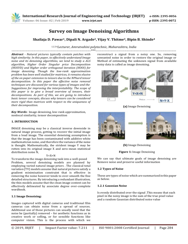
International Research Journal of Engineering and Technology (IRJET)
e-ISSN: 2395-0056
Volume: 06 Issue: 02 | Feb 2019
p-ISSN: 2395-0072
www.irjet.net
Survey on Image Denoising Algorithms
Shailaja D. Pawar1, Dipali N. Argade2, Vijay V. Thitme3, Bipin B. Shinde4
1,2,3,4Lecturer,
Amrutvahini polytechnic, Maharashtra, India
---------------------------------------------------------------------***---------------------------------------------------------------------Abstract - Natural pictures typically contain patches with
high similarity. In this paper, to effectively understand Image
noise and its denoising algorithms, we tend to study a ALS
algorithm, Higher Order Singular price Decomposition
(HOSVD) and Higher order orthogonal iteration (HOOI) for
image denoising. Though the low-rank approximation
problem has been well studied for matrices, it remains elusive
of the on paper extension to tensors due to the NPhard tensor
decomposition. In this paper the effective noise removal
techniques are discussed for various types of images and the
Suggestions for improving the interpretability. The scope of
this paper is to give a broad overview of tensors, their
decompositions. As part of this, we are going to introduce
basic tensor concepts, discuss why tensors can be considered
more rigid than matrices with respect to the uniqueness of
their decomposition.
reconstruct a signal from a noisy one. So, removing
unwanted noise in order to restore the original image or
Method of estimating the unknown signal from available
noisy data is called as image denoising.
(a) Image Denoising
Key Words: Image denoising, low-rank approximation,
nonlocal similarity, tensor decomposition
1. INTRODUCTION
IMAGE denoising may be a classical inverse downside in
natural image process, getting to recover the initial image
from a loud image. The essential denoising assumption is
that the image has been contaminated with additive white
mathematician noise, and therefore the variance of the noise
is thought. Mathematically, the strident image Y may be
rotten into its original image X and zero-mean statistical
distribution noise N,
Y=X+N
To transform the image denoising task into a well-posed
Problem, several denoising models are planned by
employing varied natural image priors . The classical total
variation (TV) models assume that natural pictures satisfy a
gradient minimisation constraint that is effective in
removing the noise however tends to over-smooth the fine
detailed structures. By introducing a redundant illustration,
the thin models assume that the clean image content can be
effectively delineated by associate degree over-complete
wordbook.
(b) Image Denoising
Figure 1: Image Denoising
We can say that ultimate goals of image denoising are
Remove noise and preserve useful information
1.2 Types of Noise
These are types of noise which are summarized in this paper
as below.
1.2.1 Gaussian Noise
Is evenly distributed over the signal .This means that each
pixel in the noisy image is the sum of the true pixel value
and a random Gaussian distributed noise value
1.1 Image Denoising:
Images captured with digital cameras and traditional film
cameras can obtain noise from a spread of sources.
Additional use of those pictures can usually need that the
noise be (partially) removed – for aesthetic functions as in
creative work or selling, or for sensible functions like
computer vision. This is the process with which we
© 2019, IRJET
|
Impact Factor value: 7.211
|
ISO 9001:2008 Certified Journal
|
Page 284
International Research Journal of Engineering and Technology (IRJET)
e-ISSN: 2395-0056
Volume: 06 Issue: 02 | Feb 2019
p-ISSN: 2395-0072
www.irjet.net
Figure 2: Gaussian Noise
1.2.2 Impulse Noise
The impulse noise is of two types, fixed value and random
value. In Fixed value i.e. Salt and pepper noise we can say
that It is generally caused due to errors in transmission and
It has only two possible values For an 8-bit image, the typical
value for pepper noise is 0 and for salt noise 255.In this the
corrupted pixels are set alternatively to minimum or to
maximum values giving the image Salt and Pepper. While in
Random value impulse noise can have any value between 0
and 255 hence its removal is very difficult.
Figure 5: Image Denoising Approaches
1.4 Image Denoising Algorithms
More than a thousand pictures are wont to do the analysis
using these CB and pellet filtering techniques to prove that
the poor quality pictures are improved terribly efficiently.
The filters area unit enhancing look of image and
additionally enhance abnormal component values. As way
strident pixels have less impact on encircled sensible ones
[5], the relation between sensible pixels and strident pixels
area unit represented. CB and pellet filters manufacture
glorious EME (Quality live of Image Enhancement), MSE,
RMSE and PSNR values compared to average filters. CB
algorithms scans all neighboring components from center
pixel for odd N x N Matrix.BB filter assigns left corner
component rather than center component and so the
scanning starts from the left corner component itself.
1.2.3 Uniform Noise
The uniform noise cause by quantizing the pixels of image
to a number of distinct levels is known as quantization
noise. Uniform noise can be analytically described by this
image.
Figure 3: Uniform Noise
1.2.4 Periodic Noise
The Source of periodic noise is from electrical or electromechanical interference during image acquisition.
Figure 4: Periodic Noise
1.3 Classification of Denoising Methods
As shown in Figure 5, there are two basic approaches to
image denoising, spatial filtering methods and transform
domain filtering methods.
© 2019, IRJET
|
Impact Factor value: 7.211
Figure 6: BB and CB Filter
|
ISO 9001:2008 Certified Journal
|
Page 285
International Research Journal of Engineering and Technology (IRJET)
e-ISSN: 2395-0056
Volume: 06 Issue: 02 | Feb 2019
p-ISSN: 2395-0072
www.irjet.net
1.4.1. Comparison between CB filter and BB Filter
1.5.3. Tensor Indexing.
Table -1: Comparison Table
We can create subarrays (or subfields) by fixing some of
the given tensor’s indices. Fibers are created when fixing
all but one index, slices (or slabs) are created when fixing
all but two indices. For a third order tensor the fibers are
given as x: jk = x jk (column), x i:k (row), and x i j: (tube); the
slices are given as X ::k = Xk (frontal), X :j: (lateral), X i::
(horizontal).Graphical examples of fibers and slices for a
3-way tensor are given in Figure 8 and 9.
1.5 Introduction to Tensors
Figure 8: Column, row, and tube fibers of a mode-3 tensor
1.5.1. Tensors
Tensors will be thought of as multi-way collections of
numbers, which generally return from a field (like R).In
the simplest high-dimensional case, such a tensor would
be a three-dimensional array, which may be thought of as
an information cube. Throughout this paper, we'll
typically seek advice from a three dimensional tensor for
motivation and ease. In most cases, the notation naturally
extends to higher-dimensional tensors. As we have a
tendency to introduce different ideas during this and also
the next sections, we'll borrow most of our notation from
the excellent review.
Figure 9:Lateral, horizontal, and frontal slices of a mode-3
Tensor
1.5.4. Outer and real number
The vector outer product is defined because the product
of the vector’s components. This operation is denoted by
the} symbol2. The vector outer product of 2 n-sized
vectors a, b is defined as follows and produces a matrix
X:X = a } b = abT
1.5.2. Tensor Order
The order1 of a tensor is that the variety of its
dimensions. Scalars will thus be taken as zeroth-order
tensors, vectors as first-order tensors, and matrices as
second-order tensors. We are going to consult with
tensors of order 3 or higher as higher order tensors.
Notation-wise, scalars are denoted by graphic symbol
letters
,
vectors
by
graphic
symbol
letters
, matrices by capital letter
,
and higher order tensors by Euler script letters
The Is denote the number of components
within the several dimension. Figure 7 shows how can we
move from scalars to tensors.
Figure 10: A rank-1 mode-3 tensor
1.6 TENSOR DECOMPOSITION ALGORITHMS
After orientating ourselves with the fundamentals of
tensors, we will now address the foremost fashionable
tensor decomposition algorithms. While this section can
offer a rather theoretical treatment, we also describe the
sensible relevancy of tensor decompositions in Section
five and Section half dozen. In specific, we have a
tendency to square measure curious whether or not we
are able to generalize the concept of the SVD from
matrices to general tensors. As we will see, there's no
single generalization of the SVD thought, but we will
discuss 2 decompositions that feature different
Figure 7:
© 2019, IRJET
|
Impact Factor value: 7.211
|
ISO 9001:2008 Certified Journal
|
Page 286
International Research Journal of Engineering and Technology (IRJET)
e-ISSN: 2395-0056
Volume: 06 Issue: 02 | Feb 2019
p-ISSN: 2395-0072
www.irjet.net
generalized properties of the matrix SVD: the canonical
polyadic decomposition (CPD) and also the Tucker
decomposition. Each square measure outer product
decompositions, but they need terribly different
structural properties. As a rule of thumb it's sometimes
suggested to use CPD for latent parameter estimation and
Tucker for mathematical space estimation, compression,
and dimensionality reduction. Since CPD and Tucker
square measure the foremost vital tensor decomposition
and many alternative decompositions square measure
supported these 2 techniques.
Algorithm 3 HOOI
Algorithm 1 ALS algorithm
Higher order orthogonal iteration (HOOI). An alternate
Approach to computing the Tucker decomposition is
provided by the higher order orthogonal iteration
(HOOI). The HOOI is actually an ALS formula that uses
the end result of playacting HOSVD on a tensor as a place
to begin for initializing the issue matrices [4]. This
formula, that is made public in formula three, is
particularly advised in cases wherever we tend to solely
have access to a truncated HOSVD, since the sequent
application of the ALS formula permits for more accurate
decompositions.
While the ALS algorithmic program printed in
algorithmic program one is straightforward to
understand and implement, it would take many steps to
converge and it would additionally not converge to a
worldwide optimum. This implies that the performance
of this algorithmic program is influenced by its
formatting.
2. CONCLUSION
We have discussed various denoising algorithms and their
performance metrics are compared with individually. The
nonlocal means with adaptability shows very good results in
image denoising. Though the applications are different, the
various denoising schemes perform within their limit. There
must be a technique which can be applied globally for all
types of noisy images irrespective of the applications. The
future research gives the scope for such denoising algorithm
which also helps in preserving the necessary sharp details of
the image.
Algorithm 2 HOSVD
REFERENCES
[1] Yue Wu, Leyuan Fang, Shutao Li “Weighted Tensor
Rank-1 Decomposition for Nonlocal Image Denoising,”
1057-7149 (c) 2018IEEE.
DOI 10.1109/TIP.2018.2889914.
Higher Order Singular price Decomposition (HOSVD). We
can currently build use of the actual fact that for a given
tensor X, we can easily find a definite Tucker
decomposition of rank ¹R1; R2; : : : ; RN ºwhere Rn =
rankn¹Xº. this offers rise to the upper order singular
value decomposition (HOSVD). The key plan behind the
HOSVD is to find the parts that best capture the variation
in mode n, while not considering the opposite modes at
now in time [38].This directly corresponds to the
essential PCA thought and may be formalized as seen in
Algorithm 2.
© 2019, IRJET
|
Impact Factor value: 7.211
[2] Prof.R.Gayathri, Dr.R.S.Sabeenian“A Survey on Image
Denoising Algorithms(IDA)”, ISSN: 2278 – 8875Vol. 1,
Issue 5, November 2012.
[3] Mukesh C. Motwani Mukesh C. Gadiya Rakhi C.
Motwani“Survey of Image Denoising Techniques”
|
ISO 9001:2008 Certified Journal
|
Page 287
International Research Journal of Engineering and Technology (IRJET)
e-ISSN: 2395-0056
Volume: 06 Issue: 02 | Feb 2019
p-ISSN: 2395-0072
www.irjet.net
[4] Brett W. Bader Tamara G. Kolda. 2009. Tensor
Decompositions and Applications. SIAM Rev. 51, 3
(August2009),455–500.
DOI:http://dx.doi.org/10.1137/07070111X
[5] Krishnan Kant Lavania, Shivali and Rajiv Kumar,”Image
Enhancement using Filtering Techniques”, International
Journal
on
computer
Science
and
Engineering,Vol.4,Issue No.1,pp.14-20, January 2012.
[6] Miguel Araujo, Spiros Papadimitriou, Stephan
Günnemann, Christos Faloutsos,Prithwish Basu,
Ananthram Swami, Evangelos E Papalexakis, and Danai
Koutra.2014. Com2: fast automatic discovery of
temporal (’Comet’) communities. InPacic-Asia
Conference on Knowledge Discovery and Data Mining.
Springer, 271–283.
[7] Hillar and L.-H. Lim. 2009. Most tensor problems are NPhard. ArXiv e-prints Nov. 2009). arXiv:cs.CC/0911.1393
[8] Ankur Padia, Kostantinos Kalpakis, and Tim Finin. 2016.
Inferring Relations in Knowledge Graphs with Tensor
Decompositions. In IEEE International Conferenceon Big
Data. IEEE.
[9] M. Protter and M. Elad, “Image sequence denoising via
sparse and redundant representations,” IEEE Trans.
Image Process., vol. 18, no.1, pp. 27-35, Jan. 2009.
© 2019, IRJET
|
Impact Factor value: 7.211
|
ISO 9001:2008 Certified Journal
|
Page 288