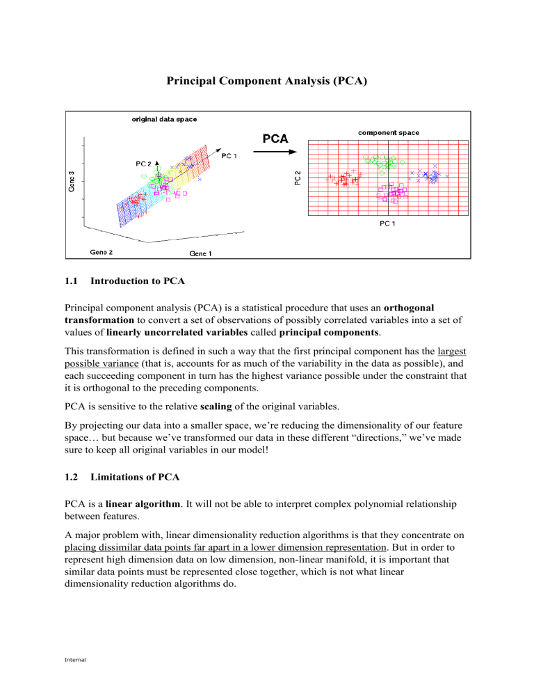
Principal Component Analysis (PCA)
1.1
Introduction to PCA
Principal component analysis (PCA) is a statistical procedure that uses an orthogonal
transformation to convert a set of observations of possibly correlated variables into a set of
values of linearly uncorrelated variables called principal components.
This transformation is defined in such a way that the first principal component has the largest
possible variance (that is, accounts for as much of the variability in the data as possible), and
each succeeding component in turn has the highest variance possible under the constraint that
it is orthogonal to the preceding components.
PCA is sensitive to the relative scaling of the original variables.
By projecting our data into a smaller space, we’re reducing the dimensionality of our feature
space… but because we’ve transformed our data in these different “directions,” we’ve made
sure to keep all original variables in our model!
1.2
Limitations of PCA
PCA is a linear algorithm. It will not be able to interpret complex polynomial relationship
between features.
A major problem with, linear dimensionality reduction algorithms is that they concentrate on
placing dissimilar data points far apart in a lower dimension representation. But in order to
represent high dimension data on low dimension, non-linear manifold, it is important that
similar data points must be represented close together, which is not what linear
dimensionality reduction algorithms do.
Internal
1.3
Eigenvectors and Eigenvalues
Eigenvectors and eigenvalues come in pairs, i.e. every eigenvector has a corresponding
eigenvalue.


Eigenvector: direction
Eigenvalue: value that describes the variance in the data in that direction
The eigenvector with the highest eigenvalue is the principal component.
The total number of eigenvector & eigenvalue sets is equal to the total number of dimensions.
2
(
2
12
3
3
3
)×( )= ( )= 4×( )
8
1
2
2
Eigenvector
1.4
Eigenvalue
Covariance
Covariance is a measure of how much two dimensions vary from their respective means with
respect to each other. The covariance of a dimension with itself is the variance of that
dimension.
𝑐𝑜𝑣(𝑋, 𝑌) =
∑𝑛𝑖=1(𝑋𝑖 − 𝑋̅)(𝑌𝑖 − 𝑌̅)
𝑛−1
The exact value of covariance is not as important as the sign of the covariance.


Internal
+ve covariance: Both dimensions increase together.
-ve covariance: Both dimensions decrease together.
1.5
Algorithm
1.5.1 Step 1 – Standardisation
For PCA to work properly, the data should be standardised/scaled. An example is to subtract
the mean from each of the data dimensions. This produces a dataset with a mean of 0.
If the importance of features is independent of the variance of the features, then divide each
observation in a column by that column’s standard deviation.
1.5.2 Step 2 – Calculate covariance matrix
𝑐𝑜𝑣(𝑥, 𝑥)
𝐶 = (𝑐𝑜𝑣(𝑦, 𝑥)
𝑐𝑜𝑣(𝑧, 𝑥)
= 𝑍𝑇 𝑍
𝑐𝑜𝑣(𝑥, 𝑦)
𝑐𝑜𝑣(𝑦, 𝑦)
𝑐𝑜𝑣(𝑧, 𝑦)
𝑐𝑜𝑣(𝑥, 𝑧)
𝑐𝑜𝑣(𝑦, 𝑧))
𝑐𝑜𝑣(𝑧, 𝑧)
1.5.3 Step 3 – Calculate the eigenvectors and eigenvalues of the covariance matrix
The eigenvectors should be unit eigenvectors, i.e. their lengths are 1. This is done by
dividing the eigenvector by its length.
This step is also known as eigendecomposition of 𝑍 𝑇 𝑍 into 𝑃𝐷𝑃−1 , where P is the matrix of
eigenvectors and D is the diagonal matrix with eigenvalues on the diagonal and values 0
elsewhere.
1.5.4 Step 4 – Choosing components and forming a feature vector
The eigenvectors are ordered according to eigenvalue, from highest to lowest. This gives the
components in the order of significance.
Now, if you like, you can decide to ignore the components of lesser significance. You do lose
some information, but if the eigenvalues are small, you don’t lose much. If you leave out
some components, the final data set will have less dimensions than the original.
Internal