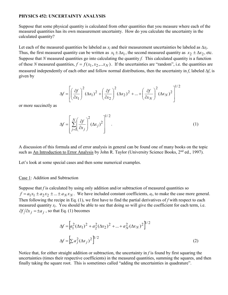
PHYSICS 452: UNCERTAINTY ANALYSIS
Suppose that some physical quantity is calculated from other quantities that you measure where each of the
measured quantities has its own measurement uncertainty. How do you calculate the uncertainty in the
calculated quantity?
Let each of the measured quantities be labeled as xj and their measurement uncertainties be labeled as xj.
Thus, the first measured quantity can be written as x1  x1 , the second measured quantity as x2  x2 , etc.
Suppose that N measured quantities go into calculating the quantity f. This calculated quantity is a function
of these N measured quantities, f  f ( x1 , x 2 ,...x N ) . If the uncertainties are “random”, i.e. the quantities are
measured independently of each other and follow normal distributions, then the uncertainty in f, labeled f, is
given by
 f  2
 f
 (x1 ) 2  
f  
 x1 
 x 2

2
 f

 (x 2 ) 2  ...  

 x N
2


 (x N ) 2 



1/ 2
or more succinctly as
1/ 2
2
N



f
2



f  
(x j )
  x j 

j

1

 

.
(1)
A discussion of this formula and of error analysis in general can be found one of many books on the topic
such as An Introduction to Error Analysis by John R. Taylor (University Science Books, 2nd ed., 1997).
Let’s look at some special cases and then some numerical examples.
Case 1: Addition and Subtraction
Suppose that f is calculated by using only addition and/or subtraction of measured quantities so
f  a1 x1  a 2 x2  ...  a N x N . We have included constant coefficients, aj, to make the case more general.
Then following the recipe in Eq. (1), we first have to find the partial derivatives of f with respect to each
measured quantity xj. You should be able to see that doing so will give the coefficient for each term, i.e.
f x j  a j , so that Eq. (1) becomes

2
f  a12 (x1 ) 2  a 22 (x2 ) 2  ...  a N
(x N ) 2

f   a 2j (x j ) 2

1/ 2

1/ 2
(2)
Notice that, for either straight addition or subtraction, the uncertainty in f is found by first squaring the
uncertainties (times their respective coefficients) in the measured quantities, summing the squares, and then
finally taking the square root. This is sometimes called “adding the uncertainties in quadrature”.
Case 2: Multiplication and Division
Suppose that f is calculated by using only multiplication of two measured quantities so f  ax1 x2 where a is
a constant. Then following the recipe in Eq. (1), we get

f  (ax 2 ) 2 (x1 ) 2  (ax1 ) 2 (x 2 ) 2

1/ 2
Dividing both sides by f gives
f  (ax 2 ) 2 (x1 ) 2 (ax1 ) 2 (x 2 ) 2 



f
 (ax1 x 2 ) 2
(ax1 x 2 ) 2 
1/ 2
 x  2  x  2 
  1    2  
 x1 
 x 2  

1/ 2
Now suppose that f is calculated by using only division of two measured quantities so f  ax1 / x2 where a
is a constant. Then following the recipe in Eq. (1), we get

f  (a / x2 ) 2 (x1 ) 2  (ax1 / x22 ) 2 (x2 ) 2

1/ 2
Dividing both sides by f gives
2 2
2
f  (a / x 2 ) 2 (x1 ) 2 (ax1 / x 2 ) (x 2 ) 



2
f
 (ax1 / x 2 ) 2

(
ax
/
x
)
1
2


1/ 2
 x  2  x  2 
  1    2  
 x1 
 x 2  

1/ 2
Notice that both the multiplication and division of the two quantities leads to the same uncertainty in f. Also
notice that in these two final equations we can identify that it is the percentage uncertainties that add in
x1
x 2
f
quadrature. That is,
is the percentage uncertainty in f, and
and
are the percentage
f
x2
x1
uncertainties in x1 and x2.
The cases that we just looked at involved only two measured quantities. One can show that for a mixture of
multiplication and division of N measured quantities one can still simply add the percentage uncertainties in
quadrature to get the percentage uncertainty of the calculated quantity. That is,
2
2
 x 2 
f  x1 
 x
  
  ..   N
 
f
 x1 
 xN
 x2 


f   x j
 
  xj
f
 



2
1/ 2



2 1 / 2

 
 
 
(3)
Example 1:
Suppose that an object is launched straight up with a spring-loaded launcher at time t = 0. With the aid of
photogates, you measure the initial velocity of the object to be vo = 8.00  0.25 m/s. You time how long it
takes the object to return to the launch point and measure t = 1.644  0.014 s. You then calculate the object’s
velocity as it strikes the launch point using v  vo  gt and obtain v = (8.0 m/s) – (9.8 m/s2)(1.644 s) = -8.11
m/s. What is the uncertainty in this velocity?
Since calculating v involves only subtraction of quantities with uncertainty, we use Eq. (2) to get

v  (vo ) 2  g 2 (t ) 2

1/ 2

 (0.25 m/s ) 2  (9.8 m/s 2 ) 2 (.014 s) 2

1/ 2
 0.93 m/s
So the final velocity is v = -8.11  0.93 m/s.
Example 2:
Suppose that the mass of an object is measured to be 0.200  0.005 kg and its velocity to be 0.25  0.01 m/s.
You calculate the object’s kinetic energy and obtain K = (1/2)mv2 = (1/2)(0.200 kg)(0.25 m/s)2 = 6.25 mJ.
What is the uncertainty in K?
Since calculating K involves only multiplication of quantities with uncertainty we can use Eq. (3). The
squaring of the speed is just a multiplication of v with itself. So we are really adding three percentage
uncertainties in quadrature: that of mass with that of speed with that of speed again. The percentage
uncertainty of mass is (m/m) = (0.005 kg)/(0.200 kg) = 2.5%. The percentage uncertainty of speed is (v/v)
= (0.01 m/s)/(0.25 m/s) = 4%. Thus, the percentage uncertainty in the kinetic energy is
2
2
K  m 
 v  

 
  2  
K  m 
 v  

1/ 2

 (2.5%) 2  2(4%) 2

1/ 2
 6.2%
Now 6.2% of 6.25 mJ is 0.39 mJ so the kinetic energy is K = 6.25  0.39 mJ.
Example 3:
Suppose that unpolarized light is passed through a linear polarizer. This light is then passed through another
linear polarizer. The angle between the polarization axes of the polarizers is measured to be  = 301.
According to the Law of Malus, one would expect the ratio of the intensity leaving the second polarizer to
the intensity entering the second polarizer to be I/Io = cos2 = cos2 (30) = 0.75. What uncertainty is there in
this ratio based upon the measurement uncertainty in the angle?
The function f in this example doesn’t involve a straight addition/subtraction or multiplication/division. But
we can still use Eq. (1). We do have to be careful and make sure that we use radians for our angle.
 = 30 = /6 and  = 1 = /180. Now f = I/Io = cos2 so

intensity ratio is ( I / I o )  4 cos 2  sin 2   () 2
The intensity ratio is I/Io = 0.75  0.015.

1/ 2

df
 -2cos sin. Thus, the uncertainty in the
d
 4 cos 2 ( / 6) sin 2 ( / 6)  ( / 180) 2

1/ 2
 0.015.