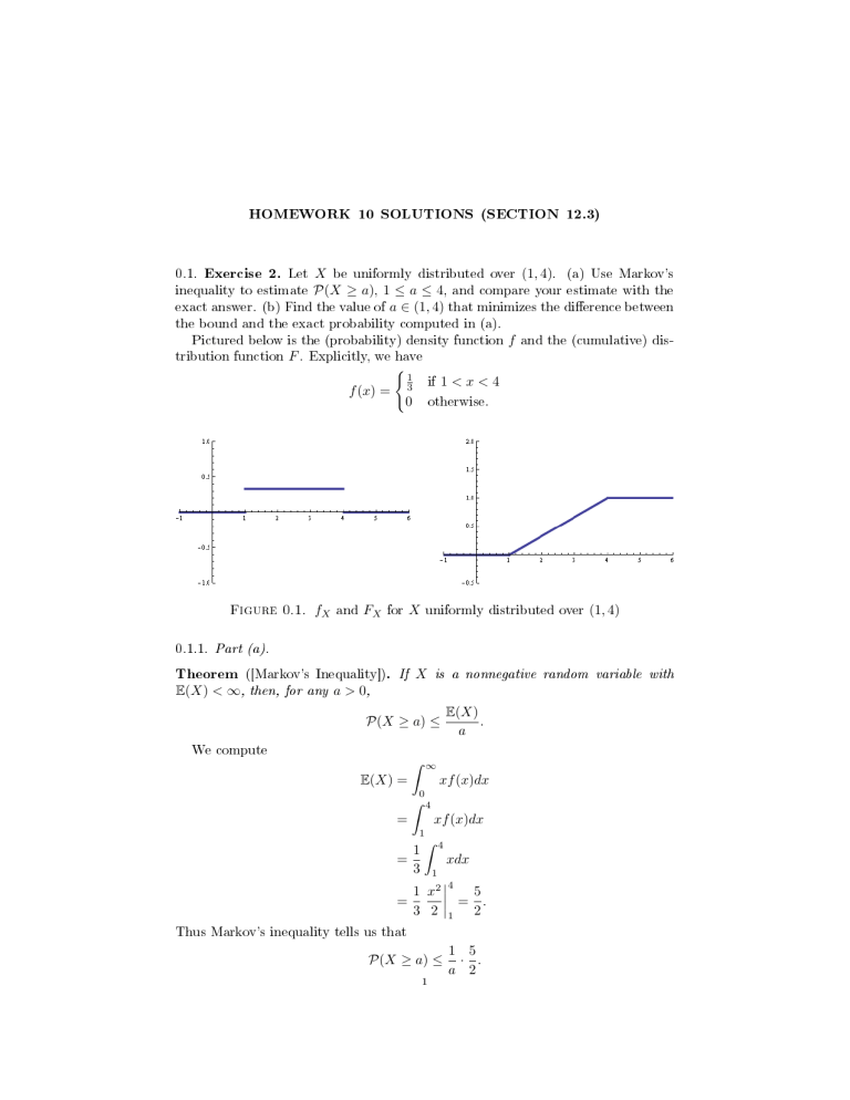
HOMEWORK 10 SOLUTIONS (SECTION 12.3)
0.1.
Exercise 2.
X be uniformly distributed over (1, 4). (a) Use Markov's
P(X ≥ a), 1 ≤ a ≤ 4, and compare your estimate with the
(b) Find the value of a ∈ (1, 4) that minimizes the dierence between
Let
inequality to estimate
exact answer.
the bound and the exact probability computed in (a).
Pictured below is the (probability) density function
tribution function
F.
(
f (x) =
Figure 0.1.
0.1.1.
f
and the (cumulative) dis-
Explicitly, we have
fX
and
FX
1
3
1<x<4
otherwise.
if
0
for
X
uniformly distributed over
(1, 4)
Part (a).
Theorem
([Markov's Inequality]).
E(X) < ∞, then, for any a > 0,
If X is a nonnegative random variable with
P(X ≥ a) ≤
We compute
ˆ
E(X)
.
a
∞
E(X) =
xf (x)dx
0
ˆ
4
=
xf (x)dx
1
=
1
3
ˆ
4
xdx
1
1 x2
=
3 2
4
=
1
5
.
2
Thus Markov's inequality tells us that
P(X ≥ a) ≤
1
1 5
· .
a 2
HOMEWORK 10 SOLUTIONS (SECTION 12.3)
In contrast, for
1 ≤ a ≤ 4,
2
we have
ˆ
∞
P(X ≥ a) =
f (x)dx
a
ˆ
4
=
a
1
dx
3
1
= (4 − a).
3
FX (a) = P(X ≤ a) = 1 − P(X ≥ a). Let's look at a table for some
1 ≤ a ≤ 4 and a graph of P(X ≥ a) and a1 · 52 . With the graph, we visually
Note that
values of
verify the application of Markov's inequality.
1
a
a
P(X ≥ a)
·
1
1
5
2
2
2
3
5
4
5
2
5
6
1
3
1
3
5
6
4
0
5
8
5
2
(a)
Comparing some
(b) Comparing P(X ≥ a) (blue) and
values.
1
a
·
5
(red)
2
Figure 0.2
0.1.2.
Part (b).
Let's dene the dierence between the functions:
g(x) =
1 5 1
· − (4 − a).
a 2 3
Next we take a derivative and solve for critical points. We have
g 0 (x) = −
5
1
+ =0
2a2
3
and solving we get
r
a=
15
.
2
Taking the second derivative we have
g 00 (x) =
which is positive for all
interval
(1, 4).
1 ≤ a ≤ 4,
and so
5
,
a3
a=
q
15
2 is a global minimum on the
HOMEWORK 10 SOLUTIONS (SECTION 12.3)
0.2.
Exercise 6.
Let
3
X be standard normally distributed. Use Chebyshev's inP(|X| ≥ 1), (b) P(|X| ≥ 2), and (c) P(|X| ≥ 3). Compare
equality to estimate (a)
each estimate with the exact answer.
Theorem
([Chebyshev's Inequality]).
If X is a random variable with nite mean
µ and nite variance σ 2 , then, for c > 0,
P (|X − µ| ≥ c) ≤
(0.1)
σ2
.
c2
Below we provide a picture (Figure 0.3) of the (probability) density function and
the cumulative distribution function of
Figure 0.3.
fX
and
FX
for
X.
X
standard normally distributed.
We we also shade the area under the probability density functions for parts (a)
and (b) (Figure 0.4).
(a) P(|X| ≥ 1)
(b) P(|X| ≥ 2)
Figure 0.4
Part (a).
1
1 = 1
(which is true for any probability). For the actual value, we use the table to get
0.2.1.
Applying 0.1 with
µ = 0, σ 2 = 1,
we have
P(|X| ≥ 1) ≤
P(|X| ≥ 1) = 2 · 0.1587 = 0.3174.
0.2.2.
Part (b).
µ = 0, σ 2 = 1, we have P(|X| ≥ 2) ≤ 14 = 0.25.
table to get P(|X| ≥ 2) = 2 · 0.0228 = 0.0456.
Applying 0.1 with
For the actual value, we use the
HOMEWORK 10 SOLUTIONS (SECTION 12.3)
0.2.3.
Part (c).
0.1111.
0.0028.
Applying 0.1 with
µ = 0, σ 2 = 1,
P(|X| ≥ 3) ≤ 19 ≈
P(|X| ≥ 3) = 2 · 0.0014 =
we have
For the actual value, we use the table to get
Remark.
4
Without using a table, we can use the 68/95/99.7% (empirical) rule to
memorize that roughly 68% of a normal distribution lies within one standard deviation of the mean, 95% within two, and 99.7% within three. Thus, roughly 32%
lies outside one, 5% lies outside two, and 0.3% lies outside three. Note that the
actual values by taking an integral are
0.31731.../0.04550.../0.00269...
0.68268.../0.95449.../0.99730...
within and
outside one/two/three standard deviations of the
mean. In a statistics book, there will be multiple tables and you can decrease the
error of your nal answer by using the proper ones.
0.3.
Exercise 12.
0.1
within
How often do you have to toss a coin to determine
P(heads)
0.9?
of its true value with probabilty at least
Method 1 (This problem is listed in 12.6.1 and so the book expects you to use
Chebyshev's inequality. For
0.3.1.
P
X n − p ≤ 0.1 ≥ 0.9
P
X n − p ≥ 0.1 ≤ 0.1.
is the same as
By Chebyshev's inequality,
σ=
p(1−p)
, and worst-case scenario is when
n
p=
1
2 , we
have
P
σ2
X n − p ≥ 0.1 ≤
0.12
=
p(1−p)
n
0.01
100
=
p(1 − p)
n 100 1
1
≤
1−
n 2
2
25
=
.
n
Thus in order to be less than
0.1,
it suces to have
25
≤ 0.1
n
or
n ≥ 250.
0.3.2.
Method 2 (Using 12.6.2).
See my Supplement to Section 12.6 for details. In
short we have
P
X n − p ≤ 0.1 ≥ 0.9
and so
P
Z≤
√
np
0.1
p(1 − p)
!
≥ 0.9
but
P (Z ≤ 1.65) = 0.9505 − 0.0495 = 0.901 > 0.9
HOMEWORK 10 SOLUTIONS (SECTION 12.3)
n
so it suces to nd
5
such that
√
Taking the worst-case scenario
np
0.1
p(1 − p)
≥ 1.65.
p, p = 12 , we have
√
1
n ≥ 16.5 ·
2
or
n ≥ 68.0625.
Notice that we don't need
n
to be nearly as large as the sucient number of
n
obtained by Chebyshev's inequality.
0.4.
Exercise 18.
1
0.5.
Exercise 23.
This wasn't one of your homeworks, but its similar to Exercise
24, and I did it above, listing it as Method 2 to Exercise 12.
0.6.
Exercise 24.
1
0.7.
Exercise 26.
1
0.8.
Exercise 28.
1
0.9.
Exercise 30.
1
0.10.
Exercise 36.
1