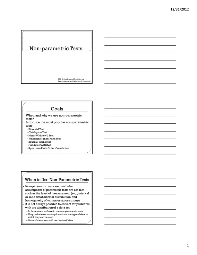
• When and why we use non-parametric tests? • Introduce the most
advertisement
12/31/2012
PSY 512: Advanced Statistics for
Psychological and Behavioral Research 2
•
•
When and why we use non-parametric
tests?
Introduce the most popular non-parametric
tests
•
•
•
•
•
•
•
•
•
Binomial Test
Chi-Square Test
Mann-Whitney U Test
Wilcoxon Signed-Rank Test
Kruskal-Wallis Test
Friedman’s ANOVA
Spearman Rank Order Correlation
Non-parametric tests are used when
assumptions of parametric tests are not met
such as the level of measurement (e.g., interval
or ratio data), normal distribution, and
homogeneity of variances across groups
It is not always possible to correct for problems
with the distribution of a data set
– In these cases we have to use non-parametric tests
– They make fewer assumptions about the type of data on
which they can be used
– Many of these tests will use “ranked” data
1
12/31/2012
The binomial
test is useful for determining if
the proportion of responses in one of two
categories is different from a specified
amount
Example: Do you prefer cats or dogs?
2
12/31/2012
The binomial test shows that the
percentage of participants selecting
“cat” or “dog” differed from .50. This
shows that participants showed a
significant preference for dogs over
cats
chi-square (χ2) statistic is a nonparametric
statistical technique used to determine if a
distribution of observed frequencies differs
from the theoretical expected frequencies
Chi-square statistics use nominal (categorical)
or ordinal level data
The
• instead of using means and variances, this test uses
frequencies.
The value of the chi-square statistic is
χ2 ∑ • Fo = Observed frequency
• Fe = Expected frequency
given by
3
12/31/2012
χ2 summarizes the discrepancies between the
expected number of times each outcome occurs and
the observed number of times each outcome occurs,
by summing the squares of the discrepancies,
normalized by the expected numbers, over all the
categories (Dorak, 2006)
Data used in a chi-square analysis has to satisfy the
following conditions
Randomly drawn from the population
Reported in raw counts of frequency
Measured variables must be independent
Observed frequencies cannot be too small (i.e., must be 5
observations or greater in each cell)
• Values of independent and dependent variables must be
mutually exclusive
•
•
•
•
There are
two types of chi-square test
• Chi-square test for goodness of fit which compares
the expected and observed values to determine how
well an experimenter's predictions fit the data
• Chi-square test for independence which compares
two sets of categories to determine whether the two
groups are distributed differently among the
categories (McGibbon, 2006)
Goodness of fit means how well a statistical model
fits a set of observations
A measure of goodness of fit typically summarize the
discrepancy between observed values and the
values expected under the model in question
The null hypothesis is that the observed values are
close to the predicted values and the alternative
hypothesis is that they are not close to the predicted
values
Example:
• Flipping a coin 100 times to determine if it is “fair”
• Observed: 47 heads and 53 tails
• Expected: 50 heads and 50 tails
4
12/31/2012
5
12/31/2012
The χ2 shows that the
observed frequencies
do not significantly
differ from the
expected frequencies
The chi-square test for independence is used to determine the
relationship between two variables of a sample. In this context
independence means that the two factors are not related.
Typically in social science research, we are interested in finding
factors that are related (e.g., education and income)
The null hypothesis is that the two variables are independent and
the alternative hypothesis is that the two variables are not
independent
• It is important to keep in mind that the chi-square test for independence
only tests whether two variables are independent or not…it cannot address
questions of which is greater or less
Example: Is the likelihood of getting into trouble in school the
same for boys and girls?
• Followed 237 elementary students for 1 semester
• Boys: 46 got into trouble and 71 did not get into trouble
• Girls: 37 got into trouble and 83 did not get into trouble
6
12/31/2012
7
12/31/2012
The χ2 shows that the two
variables are
independent such that
boys and girls are equally
likely to get into trouble
Parametric Test
Non-parametric Alternative
Two-Independent-Samples t-Test
Mann-Whitney U Test
Two-Dependent-Samples t-Test
Wilcoxon Signed-Rank Test
One-Way ANOVA
Kruskal-Wallis Test
Repeated-Measures ANOVA
Friedman’s ANOVA
Pearson Correlation or Regression
Spearman Correlation
This
is the non-parametric equivalent of the
two-independent-samples t-test
• It will allow you to test for differences
between two conditions in which different
participants have been used
This is accomplished by ranking the data
rather than using the means for each group
• Lowest score = a rank of 1
• Next highest score = a rank of 2, and so on
• Tied ranks are given the same rank: the average of the
potential ranks
• The analysis is carried out on the ranks rather than the
actual data
8
12/31/2012
•
A neurologist investigated the depressant effects of
two recreational drugs
–
–
–
–
•
Tested 20 night club attendees
10 were given an ecstasy tablet to take on a Saturday night
10 were allowed to drink only alcohol
Levels of depression were measured using the Beck
Depression Inventory (BDI) the day after (i.e., Sunday) and
four days later (i.e., Wednesday)
Rank the data ignoring the group to which a person
belonged
– A similar number of high and low ranks in each group
suggests depression levels do not differ between the groups
– A greater number of high ranks in the ecstasy group than the
alcohol group suggests the ecstasy group is more depressed
than the alcohol group
•
•
1 2 - R 1
n1 = number of participants in group 1
• Group 1 is the group with the highest summed ranks
•
•
n2 = number of participants in group 2
R1 = the sum of ranks for group 1
9
12/31/2012
•
First enter the data into SPSS
– Because the data are collected using different
participants in each group, we need to input the data
using a coding variable
• For example, create a variable called ‘Drug’ with the codes 1
(ecstasy group) and 2 (alcohol group)
•
•
There were no specific predictions about which
drug would have the most effect so the analysis
should be two-tailed
First, run some exploratory analyses on the
data
– Run these exploratory analyses for each group because
we will be looking for group differences
The KolmogorovSmirnov test (K-S test)
is a non-parametric
test for the equality of
continuous, onedimensional
probability
distributions that can
be used to compare a
sample with a
reference probability
distribution (i.e., is
the sample normally
distributed?)
The Sunday
depression data for
the Ecstasy group is
not normal which
suggests that the
sampling distribution
might also be nonnormal and that a
non-parametric test
should be used
10
12/31/2012
The Sunday
depression data for
the Alcohol group is
normal
The Wednesday
depression data for
the Ecstasy group is
normal
The Wednesday
depression data for
the Alcohol group is
not normal which
suggests that the
sampling distribution
might also be nonnormal and that a
non-parametric test
should be used
11
12/31/2012
The Shapiro-Wilk Test
also examines
whether a sample
came from a normally
distributed
population. In this
example, the results
of this test are highly
consistent with those
of the KolmogorovSmirnov Test.
However, if these two
tests differ, then you
should usually use the
Shapiro-Wilk Test
The Levene Test
compares the
variances of the
groups
The Levene Test did
not find a significant
difference in the
variance for these two
samples for the
Sunday depression
scores
12
12/31/2012
The Levene Test did
not find a significant
difference in the
variance for these two
samples for the
Wednesday
depression scores
13
12/31/2012
•
•
•
The first part of the output
summarizes the data after they
have been ranked
The second table (below) provides the actual test
statistics for the Mann-Whitney U Test and the
corresponding z-score
The significance value gives the two-tailed
probability that a test statistic of at least that
magnitude is a chance result, if the null hypothesis
is true
The Mann-Whitney U was not
significant for the Sunday data
which means that the Alcohol
and Ecstasy groups did not
differ in terms of their
depressive symptoms on
Sunday
14
12/31/2012
•
•
The second table (below) provides the actual test
statistics for the Mann-Whitney U Test and the
corresponding z-score
The significance value gives the two-tailed
probability that a test statistic of at least that
magnitude is a chance result, if the null hypothesis
is true
The Mann-Whitney U was
significant for the Wednesday
data which means that the
Alcohol and Ecstasy groups
differed in terms of their
depressive symptoms on
Wednesday
The equation to convert a z-score into the effect size
estimate r is as follows (from Rosenthal, 1991):
• z is the z-score that SPSS produces
• N is the total number of observations
• We had 10 ecstasy users and 10 alcohol users and so the total
number of observations was 20
•
Depression levels in ecstasy users (Mdn =
17.50) did not differ significantly from
alcohol users (Mdn = 16.00) the day after
the drugs were taken, U = 35.50, z = -1.11,
ns, r = -.25. However, by Wednesday, ecstasy
users (Mdn = 33.50) were significantly more
depressed than alcohol users (Mdn = 7.50),
U = 4.00, z = -3.48, p < .001, r = -.78.
15
12/31/2012
•
•
Used to compare two sets of dependent
scores (i.e., naturally occurring pairs,
researcher-produced pairs, repeated
measures)
Imagine the experimenter in the previous
example was interested in the change in
depression levels for each of the two drugs
– We still have to use a non-parametric test because
the distributions of scores for both drugs were nonnormal on one of the two days
Scores are ranked
separately for the
two groups. Scores
that did not change
(i.e., difference
score = 0) are
excluded from
ranking. Difference
scores are ranked in
terms of absolute
magnitude.
This analysis allows
us to look at the
change in
depression score for
each drug group
separately…so the
data file should be
split by drug group
(ecstasy v. alcohol)
16
12/31/2012
If you have split the file, then the first set of results
obtained will be for the ecstasy group
The Wilcoxon Signed-Rank Test was
significant for the Ecstasy group
which means that their depression
symptoms increased from Sunday to
Wednesday
The Wilcoxon SignedRank Test was
significant for the
Ecstasy group which
means that their
depression symptoms
decreased from Sunday
to Wednesday
The effect size can be calculated in the same way as for the Mann–
Whitney U Test
In this case SPSS output tells us that for the ecstasy group z is -2.53,
and for the alcohol group is -1.99.
In both cases we had 20 observations
• Although we only used 10 people and tested them twice, it is the
number of observations, not the number of people, that is
important here)
The effect size is therefore:
• .
!
"0.57
• &'('& .))
!
"0.44
17
12/31/2012
•
Reporting the values of z:
– For ecstasy users, depression levels were
significantly higher on Wednesday (M = 32.00) than
on Sunday (M = 19.60), z = -2.53, p < .05, r = -.57.
However, for alcohol users the opposite was true:
depression levels were significantly lower on
Wednesday (M = 10.10) than on Sunday (M = 16.40),
z = -1.99, p < .05, r = -.44.
•
The Kruskal-Wallis test (Kruskal & Wallis, 1952)
is the non-parametric counterpart of the oneway independent ANOVA
– If you have data that have violated an assumption then
this test can be a useful way around the problem
•
The theory for the Kruskal-Wallis test is very
similar to that of the Mann-Whitney U and
Wilcoxon test,
– Like the Mann-Whitney test, the Kruskal-Wallis test is
based on ranked data.
– The sum of ranks for each group is denoted by Ri (where
i is used to denote the particular group)
•
•
Does eating soya affect your sperm count?
Variables
– Outcome: sperm (millions)
– IV: Number of soya meals per week
• No Soya meals
• 1 soya meal
• 4 soya meals
• 7 soya meals
•
Participants
– 80 males (20 in each group)
18
12/31/2012
•
Once the sum of ranks has been calculated
for each group, the test statistic, H, is
calculated as:
– Ri is the sum of ranks for each group
– N is the total sample size (in this case 80)
– ni is the sample size of a particular group (in this
case we have equal sample sizes and they are all 20)
Run some exploratory analyses on the data
• We need to run these exploratory analyses for each group because
we’re going to be looking for group differences
The Shapiro-Wilk test
is a non-parametric
test that can be used
to compare a sample
with a reference
probability
distribution (i.e., is
the sample normally
distributed?)
19
12/31/2012
Run some exploratory analyses on the data
• We need to run these exploratory analyses for each group because
we’re going to be looking for group differences
The Shapiro-Wilk test
shows that the “no
soya” group is not
normal which
suggests that the
sampling distribution
might also be nonnormal and that a
non-parametric test
should be used
Run some exploratory analyses on the data
• We need to run these exploratory analyses for each group because
we’re going to be looking for group differences
The Shapiro-Wilk test
shows that the “1 soya
meal per week”
group is not normal
which suggests that
the sampling
distribution might
also be non-normal
and that a nonparametric test
should be used
Run some exploratory analyses on the data
• We need to run these exploratory analyses for each group because
we’re going to be looking for group differences
The Shapiro-Wilk test
shows that the “4 soya
meals per week”
group is not normal
which suggests that
the sampling
distribution might
also be non-normal
and that a nonparametric test
should be used
20
12/31/2012
Run some exploratory analyses on the data
• We need to run these exploratory analyses for each group because
we’re going to be looking for group differences
The Shapiro-Wilk test
shows that the “7 soya
meals per week”
group is normal
which suggests that a
parametric test could
be used
Run some exploratory analyses on the data
• We need to run these exploratory analyses for each group because
we’re going to be looking for group differences
The Levene test
shows that the
homogeneity of
variance assumption
has been violated
which suggests that a
non-parametric test
should be used
21
12/31/2012
The Kruskal-Wallis test
shows that there is a
difference somewhere
between the four
groups…but we need
post hoc tests to
determine where these
differences actually are
•
One way to do a non-parametric post hoc procedure is to
use Mann-Whitney tests.
– However, lots of Mann–Whitney tests will inflate the Type I error rate
• Bonferroni correction
– Instead of using .05 as the critical value for significance for each test, you use a
critical value of .05 divided by the number of tests you’ve conducted
• It is a restrictive strategy so it is a good idea to be selective about the
comparisons you make
• In this example, we have a control group which had no soya meals. As
such, a nice succinct set of comparisons would be to compare each group
against the control:
•
Comparisons:
– Test 1: one soya meal per week compared to no soya meals
– Test 2: four soya meals per week compared to no soya meals
– Test 3: seven soya meals per week compared to no soya meals
•
Bonferroni correction:
– Rather than use .05 as our critical level of significance, we’d use
.05/3 = .0167
The Mann-Whitney test
shows that there is not a
difference between the
“no soya” group and the
“1 soya meal per week”
group
22
12/31/2012
The Mann-Whitney test
shows that there is not a
difference between the
“no soya” group and the
“4 soya meals per week”
group
The Mann-Whitney test
shows that there is a
significant difference
between the “no soya”
group and the “7 soya
meals per week” group
•
For the first comparison
– (no soya vs. 1 meal) z = -0.243, the effect size is therefore:
rNoSoya-1meal •
!.*
*!
= -.04
For the second comparison
– (no soya vs. 4 meals) z = -0.325, the effect size is therefore:
rNoSoya-4meal •
!. *!
= -.05
For the third comparison
– (no soya vs. 7 meals) z = -2.597, the effect size is therefore:
rNoSoya-7meal .)+
*!
= -.41
23
12/31/2012
Used
for testing differences between
conditions when:
• There are more than two conditions
• There is dependency between the groups (naturally
occurring pairs, researcher-produced pairs, repeated
measures)
The
theory for Friedman’s ANOVA is much the
same as the other tests: it is based on ranked
data
Once the sum of ranks has been calculated for
each group, the test statistic, Fr, is calculated as:
•
•
Does the ‘Atkins’ diet work?
Variables
– Outcome: weight (Kg)
– IV: Time since beginning the diet
• Baseline
• 1 Month
• 2 Months
•
Participants
– 10 women
24
12/31/2012
The Shapiro-Wilk test
shows that the
“weight at start” is not
normally distributed
which suggests that
the sampling
distribution might
also be non-normal
and that a nonparametric test
should be used
The Shapiro-Wilk test
shows that the
“weight after 1
month” is not
normally distributed
which suggests that
the sampling
distribution might
also be non-normal
and that a nonparametric test
should be used
The Shapiro-Wilk test
shows that the
“weight after 2
months” is normally
distributed which
suggests that a
parametric test could
be used
25
12/31/2012
The omnibus ANOVA
is not significant
which suggests that
there is no difference
between the weights
of the participants at
the three time points
There is no need to
do any post hoc tests
for this example
because the omnibus
ANOVA was not
significant
For
Friedman’s ANOVA we need only report
the test statistic (χ2), its degrees of freedom
and its significance:
• The weight of participants did not significantly
change over the two months of the diet, χ2(2) = 0.20,
p > .05
26
12/31/2012
The Spearman Rank Order Correlation coefficient, rs, is a
non-parametric measure of the strength and direction of
linear association that exists between two variables
measured on at least an ordinal scale
The test is used for either ordinal variables or for interval
data that has failed the assumptions necessary for
conducting the Pearson's product-moment correlation
Assumptions:
•
•
•
•
Variables are measured on an ordinal, interval, or ratio scale
Variables do not need to be normally distributed
There is a linear relationship between the two variables
This type of correlation is not very sensitive to outliers
Example: A teacher is interested in whether those
students who do the best in Science also do the best in
Math
27
12/31/2012
The Spearman
correlation is
significant which
shows that there is a
significant linear
relationship between
science grades and
math grades for 20
elementary students
A
Spearman’s Rank Order correlation was
conducted to examine the association
between the scores of 20 elementary
students for their science and math courses.
There was a strong, positive correlation
between science and math scores which was
statistically significant (rs[18] = .94, p < .001)
28
12/31/2012
•
When data violate the assumptions of parametric tests we can
sometimes find a nonparametric equivalent
Binomial Test
•
Chi-Square Test
•
Mann-Whitney U Test
•
Wilcoxon Signed-Rank Test
•
Kruskal-Wallis Test
•
Friedman’s Test
•
Spearman’s Rank Order Correlation
•
– Compares probability of two responses
– Compares observed and expected frequencies
– Compares two independent groups of scores
– Compares two dependent groups of scores
– Compares > 2 independent groups of scores
– Compares > 2 dependent groups of scores
– Determines the strength of linear association between two variables
29
