Slide
1
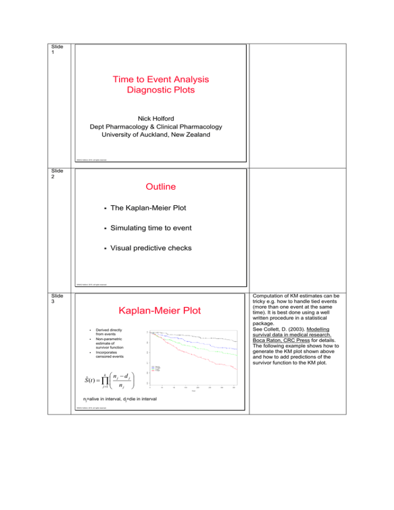
Time to Event Analysis
Diagnostic Plots
Nick Holford
Dept Pharmacology & Clinical Pharmacology
University of Auckland, New Zealand
©NHG Holford, 2015, all rights reserved.
Slide
2
Outline

The Kaplan-Meier Plot

Simulating time to event

Visual predictive checks
©NHG Holford, 2015, all rights reserved.
Slide
3
Kaplan-Meier Plot



Derived directly
from events
Non-parametric
estimate of
survivor function
Incorporates
censored events
k n d
j
j
Sˆ (t )   

n
j 1 
j




nj=alive in interval, dj=die in interval
©NHG Holford, 2015, all rights reserved.
Computation of KM estimates can be
tricky e.g. how to handle tied events
(more than one event at the same
time). It is best done using a well
written procedure in a statistical
package.
See Collett, D. (2003). Modelling
survival data in medical research.
Boca Raton, CRC Press for details.
The following example shows how to
generate the KM plot shown above
and how to add predictions of the
survivor function to the KM plot.
Slide
4
R Code for Kaplan-Meier
# Read NONMEM data file
input= "warf_sim_p1_TRT"
warf=read.csv(paste(input,".csv",sep=""),stringsAsFactors=F)
names(warf)[1]="ID" # Make a variable called ID
# Select columns to use
event = subset(warf, MDV==0,
select=c("ID","TIME","DV","TRT"))
event[,”DV”] = as.numeric(event[,”DV”])
# Run survfit() with TRT as the covariate
fit1 = survfit(Surv(TIME,DV)~TRT, data=event, conf.type="none")
©NHG Holford, 2015, all rights reserved.
Factors are a special kind of data type
that can cause problems for R
functions expecting numeric values.
By default R will treat the DV column
as a factor because the data file
contains “.” for DV when MDV=1. The
stringsAsFactors=F option is used in
read.csv() but this means all values in
the DV column will be converted to
character data type.
Then names() function is used to
rename the first variable in the warf
data frame from “_ID” to “ID”. By
default it will have the name “_ID”
because the CSV file header for the
first column is “#ID” and R converts
the “#” to “_”.
After extraction of records with events
(MDV=0) using the subset() function it
is necessary to convert the character
values of DV to numeric values for
survfit() to work properly. The
automatic conversion to factor is one
of the ‘features’ of R that often
requires the kind of workaround
shown here.
survfit() computes the non-parametric
Kaplan-Meier estimates of the
survivor function. The formula for the
survivor function includes “~TRT”
which means TRT is a covariate
distinguishing different groups so that
a separate set of KM estimates is
produced for each treatment.
Slide
5
R Code for T2E Plots
# Create plot using output from survfit()
minProb=0.6; maxTime=365
xscale = c(0,maxTime); yscale = c(minProb,1)
kmcolors=c("black","blue","green","red")
kmplot=plot(fit1,
col=kmcolors, cex.main=.95,
ylim=yscale, xlim=xscale,
xlab="Days“, ylab=paste("Prob of No Event",input)
)
legend(
legend = c("Placebo", "2.5 mg/d","5 mg/d","10 mg/d"),
lty=c(1,1,1,1),lwd=c(2,2,2,2), col=kmcolors, bty='n', cex=.8,
x=0.01*maxTime,y=minProb+(1-minProb)*0.35
)
# Add survivor function observation
pred=read.csv(“surv.csv")
lines(pred[,”time"], pred[,“mean"])
©NHG Holford, 2015, all rights reserved.
The plot() function recognizes that fit1
is an object created by survfit() and
knows how to extract the data in order
to create a line for each survivor
function and to mark censored events.
The legend() function is used to add
an informative legend to describe the
different treatments associated with
each survivor function curve.
The predicted survivor function values
from WinBugs are read using
read.csv() and overlaid on the KM plot
using the lines() function.
Slide
6
Simulating Time to Event

There is no simple solution to simulate an exact
event time

A general solution for interval censored event times
exists
» Requires pre-specifying the intervals e.g. every day for 1
year
Simulation in NONMEM is complex. The following
code snippets show some of the key features.

©NHG Holford, 2015, all rights reserved.
Slide
7
NONMEM Data Template for
Simulation of Warfarin
#ID
TIME
1
1
1
1
1
1
1
TRT
0
0
0
0
1
1
1
AMT RATE ADDL II
1
5
-2
364
1.
.
.
.
1.
.
.
.
1.
.
.
.
1.
.
.
.
1.
.
.
.
1.
.
.
.
WT
1
DVID
70
70
70
70
70
70
70
DV
0.
1.
2.
3.
1.
2.
3.
MDV
1
1
1
1
1
1
1
Data template can be used to
simulate warfarin PK (AMT, RATE,
ADDL, II) and changes in prothrombin
complex activity (PCA; DVID=1) and
international normalised ratio (INR,
DVID=2) as well as interval censored
time to event (DVID=3). Between
subject variability in warfarin PK can
be simulated in part by simulating
different weights.
©NHG Holford, 2015, all rights reserved.
Slide
8
Simulation Code 1
IF (ICALL.EQ.4) THEN
IF (NEWIND.LE.1) THEN ; first record
CALL RANDOM(2,R)
UEVT=R ; Uniform random number for event
CALL RANDOM(3,R)
UTRT=R ; Uniform random number for treatment
CALL RANDOM(3,R)
UDRP=R ; Uniform random number for dropout
IF (UTRT.LT.0.25) THEN ; placebo
RATE=0
ADDL=0
II=0
AMT=0
ELSE
©NHG Holford, 2015, all rights reserved.
This determines the random
probabilities for each subject that
determine the treatment type, the
event of interest (major bleed) and the
censoring due to random drop out.
Slide
9
Simulation Code 2
; RATE, ADDL and II are pre-specified in input data
;
RATE=-2
;
ADDL=364 ; days
;
The simulated treatments are
implemented by random assignment
of the warfarin daily dose.
Weights are simulated using a lognormal distribution for weight centered
on WT_STD with a coefficient of
variation PPV_CSV.
II=1 ; day
IF (UTRT.LT.0.5) THEN ; dose 1
AMT=2.5 ; mg
ELSE
IF (UTRT.LT.0.75) THEN ; dose 2
AMT=5 ; mg
ELSE
AMT=10 ; mg
ENDIF
ENDIF
ENDIF
SWT=WT_STD*EXP(PPV_WT) ; simulated weight
STRT=AMT ; simulated treatment
©NHG Holford, 2015, all rights reserved.
Slide
10
Simulation Code 3
Warfarin conc, PCA, cumulative
hazard of bleed (DADT(3)) and of
random drop out (DADT(4)) are
obtained by integrating this set of
differential equations.
$DES
DCP=A(1)/V
DPCA=A(2)
DINR=PCA0/DPCA
PD=1+EMAX*DCP/(C50+DCP)
DADT(1)= - CL*DCP ; warfarin conc
DADT(2)=RPCA*PD - KPCA*DPCA ; turnover for PCA
DADT(3)=HBASE*(1 + BTATRT*TRT) ; treatment is hazard predictor for bleed
DADT(4)=HDROP ; constant dropout hazard
©NHG Holford, 2015, all rights reserved.
Slide
11
Simulation Code 4
$ERROR
CP=A(1)/V
PCA=A(2)
CUMEVT=A(3) ; cumulative hazard for bleed event
CUMDRP=A(4) ; cumulative hazard for dropout event
; Prob of not having event up to this time
SEVTT=EXP(-CUMEVT) ; Survivor function (t)
; Prob of not having dropped out to this time
SDRPT=EXP(-CUMDRP) ; Survivor function (t)
©NHG Holford, 2015, all rights reserved.
Survivor function values at the time of
the NONMEM record are computed
for the event of interest (SEVTT) and
random dropout event (SDRPT).
Slide
12
Simulation Code 5
IF (ICALL.EQ.4) THEN
IF (DVID.EQ.3.AND.HASDRP.EQ.0.AND.SDRPT.LT.UDRP) THEN
HASDRP=1 ; dropout event
DVX=0 ; censored event
DVIX=3
MDVX=0
ELSE
IF (HASDRP.EQ.0.AND.HASEVT.EQ.0) THEN
IF (DVID.EQ.3) THEN ; check for event
IF (SEVTT.LT.UEVT) THEN
HASEVT=1 ; bleed event
DVX=1
DVIX=3
MDVX=0
©NHG Holford, 2015, all rights reserved.
Slide
13
Simulation Output

The NONMEM table file output is quite large
because PCA, INR and event records are
generated every day for 1 year for 1000
patients

The table file is typically post-processed e.g.
using ‘awk’ or ‘R’, to create a simulated event
data file suitable for creating KM plots or
VPCs
©NHG Holford, 2015, all rights reserved.
Slide
14
Visual Predictive Check of
Time to Event

Simulate many data sets e.g. 100

Calculate the KM survivor function estimates at each
time for each data set

Interpolate the KM survivor function at frequent
intervals e.g. every day

Calculate median and prediction intervals from the
set of interpolated KM survivor functions
©NHG Holford, 2015, all rights reserved.
Random dropout censored event and
the event of interest are simulated
here. In each case the decision to
create an event is determined by
comparing the survivor function at the
current time to the uniform random
number simulated for each subject.
Slide
15
Time to Event VPC
©NHG Holford, 2015, all rights reserved.
Slide
16
Disability Event
Final Model: time+age0+UPDRS(t)+deprenyl(t)
Without dropout
With dropout
©NHG Holford, 2015, all rights reserved.
Slide
17
Essential Reading
Collett, D. (2003). Modelling survival
data in medical research.
Boca Raton, CRC Press
Collett has a very readable style for non-statisticians. His book
is unusual because it deals extensively with parametric as well
as semi-parametric survival analysis methods.
©NHG Holford, 2015, all rights reserved.
Time to event model for disability in
Parkinson’s disease (from Vu, T. C.,
J. G. Nutt, et al. (2009). "Disease
progress and response to treatment
as predictors of survival, disability,
cognitive impairment, and depression
in Parkinson’s disease." In
Preparation.)
The VPC shows the need to include
the dropout model (due to death or
non-death random censoring) in order
to match the disability time to event
model predictions with the observed
KM survivor function estimates.