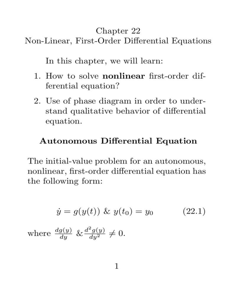
Chapter 22
Non-Linear, First-Order Differential Equations
In this chapter, we will learn:
1. How to solve nonlinear first-order differential equation?
2. Use of phase diagram in order to understand qualitative behavior of differential
equation.
Autonomous Differential Equation
The initial-value problem for an autonomous,
nonlinear, first-order differential equation has
the following form:
ẏ = g(y(t)) & y(t0 ) = y0
where
dg(y)
dy
d2 g(y)
& dy2
6= 0.
1
(22.1)
Phase Diagram
Although, it is known that solution to
(22.1) exists under the condition that dg(y)
dy
is continuous in the neighborhood around t0 ,
in most cases it is not possible to derive the
explicit solution. Often qualitative properties of the differential equation are derived by
plotting it. Such plots are known as phase
diagram.
Steps in Drawing Phase Diagram
Let the differential equation
ẏ = g(y(t)).
(22.2)
Our goal is to plot ẏ or g(y(t)).
Step 1 Take ẏ or g(y(t)) on y-axis and y(t) on
x-axis.
2
Step 2 Take the first and second derivative of ẏ
and
or g(y(t)) with respect to y, dg(y)
dy
d2 g(y)
dy 2 .
This gives you the shape of the
curve (increasing, decreasing, concave, convex).
Step 3 Derive the steady-state points by setting
ẏ = g(y(t)) = 0.
(22.3)
Steady-state or equilibrium points are the points at which the curve of ẏ or g(y)
intersects the x-axis. There can be more
than one steady-state point (multiplicity
of equilibria).
Given that there can be multiplicity of
equilibria, it raises the question which steadystate points are stable and which are unstable.
3
Stability Analysis
Stability analysis tells us about the convergence property of the differential equation.
A steady state point is stable, if the differential system converges to that point. Otherwise, it is unstable.
Theorem 22.2: A steady-state equilibrium point of a nonlinear first-order differential equation is stable if the derivative ddyẏ < 0 at that point and unstable if
the derivative is positive at that point
4
Solow or Neo-Classical Growth Model
The model relates long run per-worker consumption and growth rate in output to saving rate, work-force growth rate, and technical progress.
Assumptions
1. Constant returns to scale production technology, Y = F (K, L)
2. Diminishing Marginal Productivity of Capital
3. Constant Rate of saving (s), thus total
savings is S(t) = sY (t),
4. Constant labor force growth rate (n),
5. Constant depreciation rate (δ).
6. No technical progress (Temporary Assumption)
5
Implications of the Model
1. In the long run economy reaches a stable
steady state equilibrium.
2. Per-Worker Consumption (c) in the long
run depends on s, n, and δ. There will
be no growth in c in the long run.
3. Ultimately, an economy will grow at the
rate of work-force growth (n).
Let I(t) be gross investment, then by definition, growth rate of capital stocks is
K̇ = I(t) − δK(t).
Since in equilibrium S(t) = I(t), we have
K̇ = sY (t) − δK(t).
Now define capital-labor ratio as, κ = K
L.
Then, given constant returns to scale, perworker output, y(t) can be written as
6
Y (t)
K(t)
= F(
, 1) = f (κ(t)).
y(t) =
L(t)
L(t)
Also
K̇
sY (t) − δK(t)
=
= sy(t) − δκ(t).
L(t)
L(t)
L̇
K̇
−κ
κ̇ =
L(t)
L(t)
Combining the above two equations, we get
differential equation in the capital-labor ratio
wh- ich characterizes Solow growth model.
κ̇ = sf (κ(t)) − (δ + n)κ(t).
7
Nonautonomous and Nonlinear Equation
The general form of the nonautonomous, first-order differential equation is
ẏ = f (t, y).
(22.5)
The equation can be a nonlinear function of
both y and t. We will consider two classes of
such equations for which solutions can be easily found: Bernoulli’s Equation and Separable Equations.
Bernoulli’s Equation
The differential equation
ẏ + a(t)y = b(t)y n , n 6= 0 or 1
(22.6)
is known as Bernoulli’s Equation. Assume
that a(t) and b(t) are continuous on some
8
time interval T . Now we can transform (22.6)
as follows:
Step 1 Multiply both sides of (22.6) by y −n . We
end up with
y −n ẏ + a(t)y 1−n = b(t).
(22.7)
Step 2 Now define a new variable x = y 1−n .
Taking the derivative of x with respect
to time t, we get
ẋ = (1 − n)y −n ẏ.
(22.8)
Step 3 Using the definition in step 2, differential
equation (22.7) can be written as
ẋ + (1 − n)a(t)x = (1 − n)b(t).
9
(22.9)
This is first-order linear nonautonomous differential equation, which can be solved by using techniques learned in the
previous chapter.
Step 4 Once we have solved for x(t), we make
use of definition in step 2, x = y 1−n and
derive the solution for y(t).
Remark: This procedure is valid only when
y(t) 6= 0 forall t ∈ T .
10
Solow Growth Model With Technical Change
Earlier, we considered Solow growth model without technical change. Now, we introduce technical change. Now suppose that
production depends on capital, k, and effective labor, EL defined as
EL(t) = E(t)L(t)
where E(t) is a measure of technology. Suppose E(t) evolves as follows
Ė = λE(t), λ > 0.
Such technical change is called labor augmenting. Production function is
Y (t) = F (K(t), EL(t)) = K(t)α EL(t)1−α .
Rest of the model is identical to the previous
one. Now define capital-effective labor ratio
11
K
as, κ = EL
. Then, given constant returns to
scale, output per effective labor unit, y(t) can
be written as
Y (t)
K(t)
y(t) =
= F(
, 1) = κ(t)α .
EL(t)
EL(t)
Also
sY (t) − δK(t)
K̇
=
= sy(t) − δκ(t).
EL(t)
EL(t)
ĖL
K̇
−κ
κ̇ =
EL(t)
EL(t)
Combining the above two equations, we get
differential equation in capital-effective labor
ratio which characterizes Solow growth model
with technical change.
κ̇ + (δ + λ + n)κ(t) = sκ(t)α .
12
As we can see that it is a Bernoulli equation.
In order to solve this multiply both sides by
κ−α and define x = κ1−α . Then the above
equation can be transformed into
ẋ + (δ + λ + n)(1 − α)x(t) = (1 − α)s.
The solution is
s
x(t) =
+ C exp−(δ+λ+n)(1−α)t .
δ+λ+n
In terms of κ(t), we get
κ(t) =
·
s
+ C exp−(δ+λ+n)(1−α)t
δ+λ+n
Steady-state κ(t) is given by
·
s
κ=
δ+λ+n
13
1
¸ 1−α
.
1
¸ 1−α
.
Implications
1. Ultimately economy reaches steady-state
just as in case of no technical progress.
2. At the steady state output, Y , consumption, C, and capital stock, K, grow at
the rate of λ + n.
3. At the steady state per-worker output,
Y
C
,
consumption
per
worker,
L
L , and capital stock per worker, K
L , grow at the rate
of λ.
14
Separable Equations
The nonautonomous equation is
ẏ = f (t, y).
(22.10)
f (t, y) can always be written as the ratio of
two other functions, M (t, y), and −N (t, y).
We can then rewrite (22.10) as
M (t, y) + N (t, y)ẏ = 0.
(22.11
Definition : A non-linear, first-order
differential equation is separable if
M (t, y) = A(t), a function of only t, and
N (t, y) = y, a function of only y. A separable, nonlinear, first-order differential
equation can therefore be written as
A(t) + b(y)ẏ = 0.
(22.12)
(22.12) can be solved by direct integration.
(22.12) can be written as
15
A(t)dt + b(y)dy = 0.
(22.13)
This equation can be integrated directly to
obtain
Z
Z
A(t)dt +
b(y)dy = C.
16
(22.14)