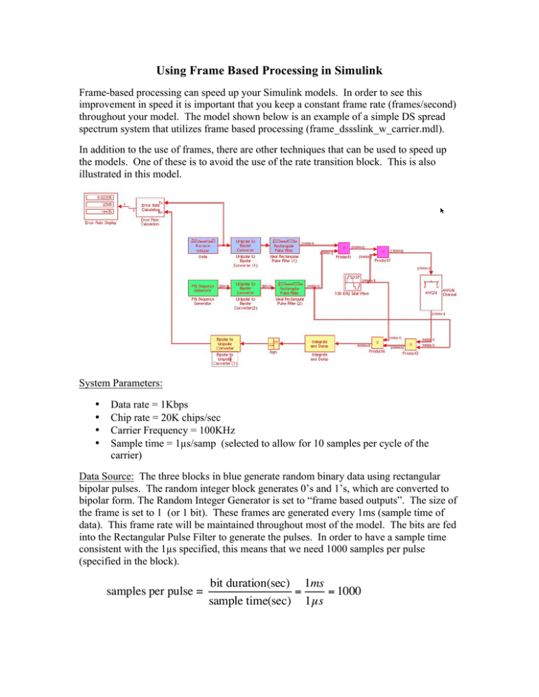
Using Frame Based Processing in Simulink
Frame-based processing can speed up your Simulink models. In order to see this
improvement in speed it is important that you keep a constant frame rate (frames/second)
throughout your model. The model shown below is an example of a simple DS spread
spectrum system that utilizes frame based processing (frame_dssslink_w_carrier.mdl).
In addition to the use of frames, there are other techniques that can be used to speed up
the models. One of these is to avoid the use of the rate transition block. This is also
illustrated in this model.
System Parameters:
•
•
•
•
Data rate = 1Kbps
Chip rate = 20K chips/sec
Carrier Frequency = 100KHz
Sample time = 1µs/samp (selected to allow for 10 samples per cycle of the
carrier)
Data Source: The three blocks in blue generate random binary data using rectangular
bipolar pulses. The random integer block generates 0’s and 1’s, which are converted to
bipolar form. The Random Integer Generator is set to “frame based outputs”. The size of
the frame is set to 1 (or 1 bit). These frames are generated every 1ms (sample time of
data). This frame rate will be maintained throughout most of the model. The bits are fed
into the Rectangular Pulse Filter to generate the pulses. In order to have a sample time
consistent with the 1µs specified, this means that we need 1000 samples per pulse
(specified in the block).
samples per pulse =
bit duration(sec) 1ms
=
= 1000
sample time(sec) 1µs
The resulting 1000 samples per bit are in a frame of size 1000 x 1. Note the settings used
in this block to create pulses with amplitude 1.
Chip Generator: The three blocks in green generate chips in a pseudo-random sequence
in a manner similar to the data source above. In order to generate frames of length 1000
at a rate of 1 frame per millisecond, we start by generating the PN sequence in frames of
length 20:
number of chips per frame =
chip rate(chips/sec)
20000
=
= 20
frame rate(frames/sec) 1000
In order to sample the chips at the same rate as the data pulses:
samples per chip =
chip duration(sec) 1 / 20000
=
= 50
sample time(sec)
1µs
We set the Rectangular Pulse Filter accordingly. Again, note the settings used to obtain
pulses with amplitude 1. This results in chips generated in frames of length 1000, the
same as the data frames. It is important that they are the same length since they are
combined in a number of mathematical operations.
Carrier: The carrier is generated with a sine wave source. It is important to use the sine
wave source that is part of the Signal Processing Blockset, since this has the option of
generating frames. This block is set to generate a 100KHz sine wave with a sample rate
of 1µs (as above) and 1000 samples per frame. Again:
1
sample time(sec/sample)*samples/frame
1
=
= 1000
1µs *1000
frame rate(frames/sec) =
or 1mS/frame. Again, is it important that the frames are of length 1000.
The remainder of the model is similar to the sample based DS spread spectrum system.
Note that there are no delays introduced in the system. Thus, the receive delay set in the
Error Rate Calculation Block is zero. Run this simulation for 100000mS (100000 bits).
Note how quickly the model runs in comparison to the sample-based model.
In this simple model it was possible to keep the frame size (and sample rate) consistent
throughout most of the model. In more complex models you may need to use multiple
sample rates. You can do this with frame based processing and still keep the frame rate
constant by changing the number of samples per frame. Blocks are available for up and
down sampling to accomplish this.
It is recommended that you select: Format à Port/Signal Displays à Signal Dimensions
so that you can observe the frame sizes throughout the model. Note that the double line
indicates that we have frames. After the Integrate and Dump block, the number of
samples per frame has reduced to 1. Thus, the size is not shown. However, the double
line is still shown to indicate that we are using frames (1 x 1).
Turning on Format à Sample Time Display à Colors will show that the frame rate is
constant throughout the model.