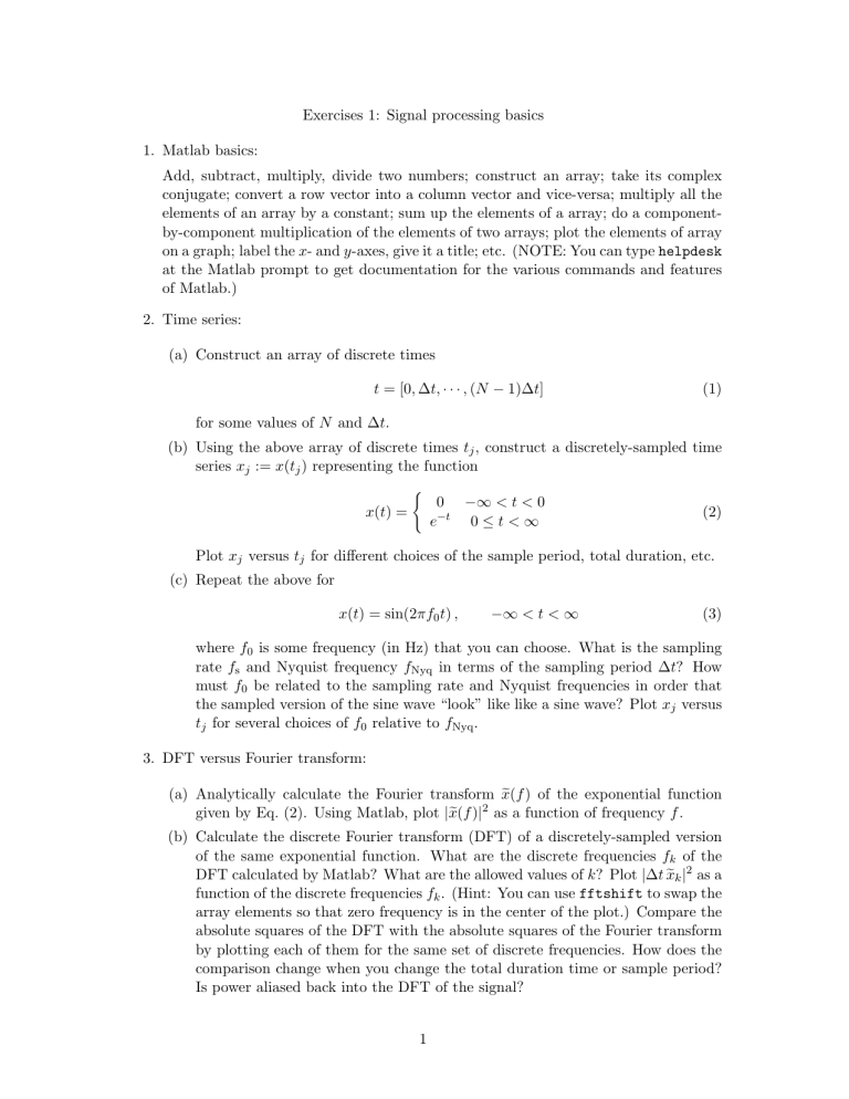
Exercises 1: Signal processing basics
1. Matlab basics:
Add, subtract, multiply, divide two numbers; construct an array; take its complex conjugate; convert a row vector into a column vector and vice-versa; multiply all the elements of an array by a constant; sum up the elements of a array; do a componentby-component multiplication of the elements of two arrays; plot the elements of array on a graph; label the x - and y -axes, give it a title; etc. (NOTE: You can type helpdesk at the Matlab prompt to get documentation for the various commands and features of Matlab.)
2. Time series:
(a) Construct an array of discrete times t = [0 , ∆ t, · · · , ( N − 1)∆ t ] (1) for some values of N and ∆ t .
(b) Using the above array of discrete times t j
, construct a discretely-sampled time series x j
:= x ( t j
) representing the function x ( t ) =
(
0 −∞ < t < 0 e
− t
0 ≤ t < ∞
(2)
Plot x j versus t j for different choices of the sample period, total duration, etc.
(c) Repeat the above for x ( t ) = sin(2 πf
0 t ) , −∞ < t < ∞ (3) where f
0 is some frequency (in Hz) that you can choose. What is the sampling rate f s must f
0 and Nyquist frequency f
Nyq in terms of the sampling period ∆ t ? How be related to the sampling rate and Nyquist frequencies in order that the sampled version of the sine wave “look” like like a sine wave? Plot x j versus t j for several choices of f
0 relative to f
Nyq
.
3. DFT versus Fourier transform:
(a) Analytically calculate the Fourier transform given by Eq. (2). Using Matlab, plot | x ( f ) | 2 e x e
( f ) of the exponential function as a function of frequency f .
(b) Calculate the discrete Fourier transform (DFT) of a discretely-sampled version of the same exponential function. What are the discrete frequencies f k of the
DFT calculated by Matlab? What are the allowed values of k ? Plot | ∆ t x e k
| 2 as a function of the discrete frequencies f k
. (Hint: You can use fftshift to swap the array elements so that zero frequency is in the center of the plot.) Compare the absolute squares of the DFT with the absolute squares of the Fourier transform by plotting each of them for the same set of discrete frequencies. How does the comparison change when you change the total duration time or sample period?
Is power aliased back into the DFT of the signal?
1

(c) Repeat the above two parts for the sinusoidal function given by Eq. (3) for several values of f
0
, some greater and some less than the Nyquist critical frequency f
Nyq
.
Also, choose some of the values of f
0 to coincide (and not to coincide) with one of the discrete frequencies f k
. How do the absolute squares of the DFT and
Fourier transform compare for the different values of power aliased back into the DFT of the signal?
f
0
? When f
0
> f
Nyq
, is
4. Parseval’s theorem:
Using the exponential and sinusoidal functions defined above (or any other functions that you’d like to construct), check the discretised version of Parseval’s theorem
N − 1
X
| x j
|
2 j =0
1
=
N
N/ 2 − 1
X k = − N/ 2
| x e k
|
2
(4)
5. Windowing:
(a) Type help window at the Matlab prompt to get a listing of the different types of window functions available in Matlab. Generate a few such windows and plot them on the same figure to get a feel of their similarities and differences.
(b) Compare the DFT of a time series x j both | x e k
| 2 and | y e k
| 2 with and without windowing, by plotting as functions of the discrete frequencies f k
, where y e k is the
DFT of the windowed data y j
:= x j w j and w j are the discrete values of some window function. NOTE: To get the amplitudes to come out right, you will need to divide | y e k
| 2 by a factor
W ss
:=
1
N
N − 1
X w
2 j
(5) j =0 to account for the reduction in the amplitude of the time series values due to the windowing.
2