Chapter 65
Linear regression
65.1 Introduction to linear
regression
Regression analysis, usually termed regression, is used
to draw the line of ‘best fit’ through co-ordinates on a
graph. The techniques used enable a mathematical equation of the straight line form y = mx + c to be deduced
for a given set of co-ordinate values, the line being such
that the sum of the deviations of the co-ordinate values
from the line is a minimum, i.e. it is the line of ‘best
fit’. When a regression analysis is made, it is possible to
obtain two lines of best fit, depending on which variable
is selected as the dependent variable and which variable
is the independent variable. For example, in a resistive
electrical circuit, the current flowing is directly proportional to the voltage applied to the circuit. There are
two ways of obtaining experimental values relating the
current and voltage. Either, certain voltages are applied
to the circuit and the current values are measured, in
which case the voltage is the independent variable and
the current is the dependent variable; or, the voltage can
be adjusted until a desired value of current is flowing
and the value of voltage is measured, in which case the
current is the independent value and the voltage is the
dependent value.
65.2 The least-squares regression
lines
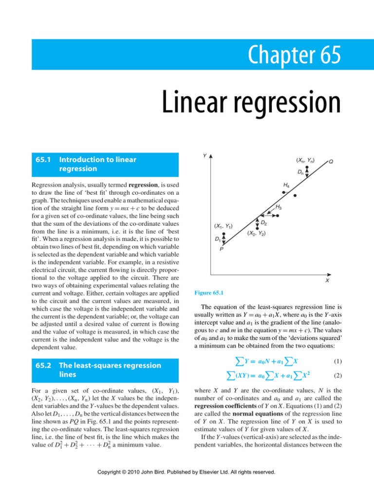
For a given set of co-ordinate values, (X1 , Y1 ),
(X2 , Y2 ), . . . , (Xn , Yn ) let the X values be the independent variables and the Y -values be the dependent values.
Also let D1 , . . . , Dn be the vertical distances between the
line shown as PQ in Fig. 65.1 and the points representing the co-ordinate values. The least-squares regression
line, i.e. the line of best fit, is the line which makes the
value of D12 + D22 + · · · + Dn2 a minimum value.
Y
(Xn, Yn)
Q
Dn
H4
H3
(X1, Y1)
D2
(X2, Y2)
D1
P
X
Figure 65.1
The equation of the least-squares regression line is
usually written as Y = a0 + a1 X, where a0 is the Y -axis
intercept value and a1 is the gradient of the line (analogous to c and m in the equation y = mx + c). The values
of a0 and a1 to make the sum of the ‘deviations squared’
a minimum can be obtained from the two equations:
Y = a0 N + a1 X
(1)
(XY) = a0 X + a1 X 2
(2)
where X and Y are the co-ordinate values, N is the
number of co-ordinates and a0 and a1 are called the
regression coefficients of Y on X. Equations (1) and (2)
are called the normal equations of the regression line
of Y on X. The regression line of Y on X is used to
estimate values of Y for given values of X.
If the Y -values (vertical-axis) are selected as the independent variables, the horizontal distances between the
Copyright © 2010 John Bird. Published by Elsevier Ltd. All rights reserved.
Linear regression 7
line shown as PQ in Fig. 65.1 and the co-ordinate values
(H3 , H4 , etc.) are taken as the deviations. The equation
of the regression line is of the form: X = b0 + b1 Y and
the normal equations become:
X = b0 N + b1 Y
(3)
(XY) = b0 Y + b1 Y 2
(4)
where X and Y are the co-ordinate values, b0 and b1
are the regression coefficients of X on Y and N is the
number of co-ordinates. These normal equations are of
the regression line of X on Y , which is slightly different
to the regression line of Y on X. The regression line of
X on Y is used to estimate values of X for given values
of Y . The regression line of Y on X is used to determine
any value of Y corresponding to a given value of X. If
the value of Y lies within the range of Y -values of the
extreme co-ordinates, the process of finding the corresponding value of X is called linear interpolation. If
it lies outside of the range of Y -values of the extreme
co-ordinates then the process is called linear extrapolation and the assumption must be made that the line of
best fit extends outside of the range of the co-ordinate
values given.
By using the regression line of X on Y , values of X
corresponding to given values of Y may be found by
either interpolation or extrapolation.
65.3 Worked problems on linear
regression
Problem 1. In an experiment to determine the
relationship between frequency and the inductive
reactance of an electrical circuit, the following
results were obtained:
Since the regression line of inductive reactance on frequency is required, the frequency is the independent
variable, X, and the inductive reactance is the dependent variable, Y . The equation of the regression line of
Y on X is:
Y = a0 + a1 X
and the regression coefficients a0 and a1 are obtained
by using the normal equations
Y = a0 N + a1
X
and
XY = a0
X + a1
X2
(from equations (1) and (2))
A tabular approach is used to determine the summed
quantities.
Frequency, X
Inductive
reactance, Y
X2
50
30
2500
100
65
10 000
150
90
22 500
200
130
40 000
250
150
62 500
300
190
90 000
350
X = 1400
200
Y = 855
122 500
2
X = 350 000
Y2
XY
Frequency (Hz)
50
100
150
1500
900
Inductive
reactance (ohms)
30
65
90
6500
4225
13 500
8100
200
250
300
350
26 000
16 900
Inductive
130
reactance (ohms)
150
190
200
37 500
22 500
57 000
36 100
70 000
40 000
Frequency (Hz)
Determine the equation of the regression line of
inductive reactance on frequency, assuming a linear
relationship.
XY = 212 000
Copyright © 2010 John Bird. Published by Elsevier Ltd. All rights reserved.
Y 2 = 128 725
8 Engineering Mathematics
The number of co-ordinate values given, N is 7.
Substituting in the normal equations gives:
855 = 7a0 + 1400a1
212 000 = 1400a0 + 350 000a1
(2)
(3)
(4)
(4)–(3) gives:
287 000 = 0 + 490 000a1
(5)
287 000
= 0.586
490 000
Substituting a1 = 0.586 in equation (1) gives:
from which, a1 =
855 = 7a0 + 1400(0.586)
i.e.
a0 =
855 − 820.4
= 4.94
7
Thus the equation of the regression line of inductive
reactance on frequency is:
Y = 4.94 + 0.586X
Problem 2. For the data given in Problem 1,
determine the equation of the regression line of
frequency on inductive reactance, assuming a linear
relationship
In this case, the inductive reactance is the independent
variable X and the frequency is the dependent variable
Y . From equations 3 and 4, the equation of the regression
line of X on Y is:
X = b0 + b1 Y
and the normal equations are
X = b0 N + b1
Y
and
XY = b0
Y + b1
Y2
From the table shown in Problem 1, the simultaneous
equations are:
1400 = 7b0 + 855b1
212 000 = 855b0 + 128 725b1
and
b1 = 1.69, correct to 3 significant figures.
Thus the equation of the regression line of frequency on
inductive reactance is:
7 × (2) gives:
1 484 000 = 9800a0 + 2 450 000a1
b0 = −6.15
(1)
1400 × (1) gives:
1 197 000 = 9800a0 + 1 960 000a1
Solving these equations in a similar way to that in
problem 1 gives:
X = −6.15 + 1.69Y
Problem 3. Use the regression equations
calculated in Problems 1 and 2 to find (a) the value
of inductive reactance when the frequency is
175 Hz, and (b) the value of frequency when the
inductive reactance is 250 ohms, assuming the line
of best fit extends outside of the given co-ordinate
values. Draw a graph showing the two regression
lines
(a) From Problem 1, the regression equation of inductive reactance on frequency is:
Y = 4.94 + 0.586X. When the frequency, X, is
175 Hz, Y = 4.94 + 0.586(175) = 107.5, correct
to 4 significant figures, i.e. the inductive reactance
is 107.5 ohms when the frequency is 175 Hz.
(b) From Problem 2, the regression equation of frequency on inductive reactance is:
X = −6.15 + 1.69Y . When the inductive reactance, Y , is 250 ohms, X = −6.15 + 1.69(250) =
416.4 Hz, correct to 4 significant figures, i.e.
the frequency is 416.4 Hz when the inductive
reactance is 250 ohms.
The graph depicting the two regression lines is shown
in Fig. 65.2. To obtain the regression line of inductive reactance on frequency the regression line equation
Y = 4.94 + 0.586X is used, and X (frequency) values of
100 and 300 have been selected in order to find the corresponding Y values. These values gave the co-ordinates
as (100, 63.5) and (300, 180.7), shown as points A
and B in Fig. 65.2. Two co-ordinates for the regression
line of frequency on inductive reactance are calculated
using the equation X = −6.15 + 1.69Y , the values of
inductive reactance of 50 and 150 being used to obtain
the co-ordinate values. These values gave co-ordinates
(78.4, 50) and (247.4, 150), shown as points C and D
in Fig. 65.2.
It can be seen from Fig. 65.2 that to the scale drawn,
the two regression lines coincide. Although it is not
necessary to do so, the co-ordinate values are also shown
to indicate that the regression lines do appear to be the
Copyright © 2010 John Bird. Published by Elsevier Ltd. All rights reserved.
Linear regression 9
Y
Using a tabular approach to determine the
values of the summations gives:
Inductive reactance in ohms
300
250
Radius, X
200
B
D
150
100
A
50
0
55
5
3025
30
10
900
16
15
256
12
20
144
11
25
121
9
30
81
7
35
49
5
40
C
100
200 300 400
Frequency in hertz
X
500
Figure 65.2
lines of best fit. A graph showing co-ordinate values is
called a scatter diagram in statistics.
X = 145
Force (N)
25
2
X = 4601
Y = 180
Y2
XY
Problem 4. The experimental values relating
centripetal force and radius, for a mass travelling at
constant velocity in a circle, are as shown:
275
25
300
100
240
225
240
400
275
625
270
900
245
1225
200
1600
5 10 15 20 25 30 35 40
Radius (cm) 55 30 16 12 11
9
7
5
Determine the equations of (a) the regression line
of force on radius and (b) the regression line of
force on radius. Hence, calculate the force at a
radius of 40 cm and the radius corresponding to a
force of 32 N
Let the radius be the independent variable X, and the
force be the dependent variable Y . (This decision is
usually based on a ‘cause’ corresponding to X and an
‘effect’ corresponding to Y .)
(a) The equation of the regression line of force on
radius is of the form Y = a0 + a1 X and the constants a0 and a1 are determined from the normal
equations:
and
X2
Force, Y
X
Y = a0 N + a1
XY = a0
X + a1
X2
(from equations (1) and (2))
Thus
and
XY = 2045
Y 2 = 5100
180 = 8a0 + 145a1
2045 = 145a0 + 4601a1
Solving these simultaneous equations gives
a0 = 33.7 and a1 = −0.617, correct to 3 significant figures. Thus the equation of the regression
line of force on radius is:
Y = 33.7 − 0.617X
Copyright © 2010 John Bird. Published by Elsevier Ltd. All rights reserved.
10 Engineering Mathematics
(b) The equation of the regression line of radius on
force is of the form X = b0 + b1 Y and the constants b0 and b1 are determined from the normal
equations:
Y
X = b0 N + b1
and
XY = b0
Y + b1
Y2
(from equations (3) and (4))
The values of the summations have been obtained
in part (a) giving:
145 = 8b0 + 180b1
and
X = 44.2 − 1.16Y
The force, Y , at a radius of 40 cm, is obtained
from the regression line of force on radius, i.e.
Y = 33.7 − 0.617(40) = 9.02,
i.e. the force at a radius of 40 cm is 9.02 N
The radius, X, when the force is 32 Newton’s
is obtained from the regression line of radius on
force, i.e. X = 44.2 − 1.16(32) = 7.08,
i.e. the radius when the force is 32 N is 7.08 cm
Now try the following exercise
Exercise 222 Further problems on linear
regression
In Problems 1 and 2, determine the equation of the
regression line of Y on X, correct to 3 significant
figures.
X
Y
14
900
18
1200
23
1600
30
2100
50
3800
[Y = −256 + 80.6X]
2.
3. The data given in Problem 1.
[X = 3.20 + 0.0124Y ]
4. The data given in Problem 2.
[X = −0.056 + 4.56Y ]
5. The relationship between the voltage applied
to an electrical circuit and the current flowing
is as shown:
Current
(mA)
2045 = 180b0 + 5100b1
Solving these simultaneous equations gives
b0 = 44.2 and b1 = −1.16, correct to 3 significant
figures. Thus the equation of the regression line of
radius on force is:
1.
In Problems 3 and 4, determine the equations
of the regression lines of X on Y for the data
stated, correct to 3 significant figures.
X 6
3
9
15 2
14 21 13
Y 1.3 0.7 2.0 3.7 0.5 2.9 4.5 2.7
[Y = 0.0477 + 0.216X]
2
4
6
8 10 12 14
Applied
voltage (V) 5 11 15 19 24 28 33
Assuming a linear relationship, determine the
equation of the regression line of applied voltage, Y , on current, X, correct to 4 significant
figures.
[Y = 1.142 + 2.268X]
6. For the data given in Problem 5, determine the
equation of the regression line of current on
applied voltage, correct to 3 significant figures.
[X = −0.483 + 0.440Y ]
7. Draw the scatter diagram for the data given
in Problem 5 and show the regression lines
of applied voltage on current and current on
applied voltage. Hence determine the values
of (a) the applied voltage needed to give a
current of 3 mA and (b) the current flowing
when the applied voltage is 40 volts, assuming
the regression lines are still true outside of the
range of values given.
[(a) 7.92 V (b) 17.1 mA]
8. In an experiment to determine the relationship
between force and momentum, a force, X, is
applied to a mass, by placing the mass on an
inclined plane, and the time, Y , for the velocity
to change from u m/s to v m/s is measured. The
results obtained are as follows:
Force (N)
Time (s)
11.4
18.7
0.56
Copyright © 2010 John Bird. Published by Elsevier Ltd. All rights reserved.
0.35
11.7
0.55
Linear regression 11
Force (N) 12.3 14.7 18.8 19.6
Time (s)
0.52 0.43 0.34 0.31
Determine the equation of the regression line
of time on force, assuming a linear relationship
between the quantities, correct to 3 significant
figures.
[Y = 0.881 − 0.0290X]
10. Draw a scatter diagram for the data given in
Problem 8 and show the regression lines of
time on force and force on time. Hence find
(a) the time corresponding to a force of 16 N,
and (b) the force at a time of 0.25 s, assuming
the relationship is linear outside of the range
of values given.
[(a) 0.417 s (b) 21.7 N]
9. Find the equation for the regression line of
force on time for the data given in Problem 8,
correct to 3 decimal places.
[X = 30.194 − 34.039Y ]
Copyright © 2010 John Bird. Published by Elsevier Ltd. All rights reserved.


