RC Filters
TEP
Related Topics
High-pass, low-pass, Wien-Robinson bridge, parallel-T filters, differentiating network, integrating network, step response, square wave, transfer function.
Principle
Resistor-Capacitor (RC) circuits serve as filters for frequencies. The frequency response of the most
commonly used RC filters is recorded by point-by-point measurements as well as the frequency sweep
method, and displayed on the oscilloscope. The results are plotted and verified using the “measure”
analysis software.
Equipment
1 Plug- in board, 4 mm plugs
1 Resistor in plug- in box, 500 Ohms
4 Capacitor/case 1/10 nF
5 Carbon resistor 1 W, 1 kOhm
5 Connect. plug white 19 mm pitch
1 Difference amplifier
1 Digital function generator
1 25 MHz Digital storage oscilloscope
Alternative for 25 MHz Digital storage oscilloscope:
1 Oscilloscope 30 MHz, 2 channels
2 Adapter; BNC- plug/socket 4 mm
1 Adapter, BNC T-plug/socket 4 mm
1 Connecting cord, l = 100 mm, yellow
2 Connecting cord, l = 500 mm, red
3 Connecting cord, l = 500 mm, blue
1 Measurement software “Measure”
1 Screened cable, BNC, l = 300 mm
1 Screened cable, BNC, l = 1500 mm
06033-00
06057-50
39105-14
39104-19
39170-00
11444-93
13654-99
11456-99
11459-95
07542-26
07542-21
07359-02
07361-01
07361-04
14500-00
07542-10
07542-12
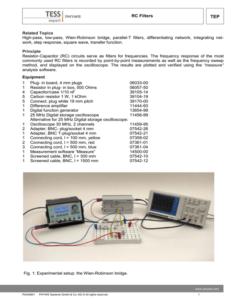
Fig. 1: Experimental setup: the Wien-Robinson bridge.
www.phywe.com
P2440801
PHYWE Systeme GmbH & Co. KG © All rights reserved
1
RC Filters
TEP
Tasks
Record the frequency response of the output voltage of
1. a high-pass filter
2. a low-pass filter
3. a band-pass filter
4. a Wien-Robinson bridge
-
5. a parallel-T filter, point by point and to display the sweep on the oscilloscope.
Investigate the step response of
6. a differentiating network
7. an integrating network
-
Analyze and verify the measurements using the “measure” analysis software.
Set-up and Procedure
Set up the experiment in accordance with Fig. 1 or the circuit diagrams in Figs. 2 to 6. To measure
the frequency response point by point, the input and output voltages U i and U O are measured with
the oscilloscope. Split the generator signal with the BNC T-plug, as seen in Fig. 1. Connect one output directly to one of the oscilloscope channels, and the other through the analyzed circuit to the
other oscilloscope channel. Adjust the oscilloscope channel settings to properly see both signals on
the display.
Fig. 2: High-pass filter.
Fig. 3: Low-pass filter.
2
P2440801
PHYWE Systeme GmbH & Co. KG © All rights reserved
RC Filters
TEP
Fig. 4: Band-pass filter.
Fig. 5: Wien-Robinson bridge.
Fig. 6: Parallel T-filter.
www.phywe.com
P2440801
PHYWE Systeme GmbH & Co. KG © All rights reserved
3
RC Filters
TEP
-
The frequency response can also be displayed on the oscilloscope by sweeping the generator frequency. In this case the U~f-output of the generator is connected to the X-input of the oscilloscope
in X-Y operation (channel 1), while the signal passing through the circuit setup is connected to the
Y-input of the oscilloscope (channel 2). Set the generator function to the f 1 …f 2 mode and a logarithmic range with adequate sweep factor (f n =f n −1 *sweep factor). Enter the desired values for the fre-
quency range (f 1 and f 2 ) and choose the f 1 …f 2 mode from the U~f menu. The menu contains
some preset frequency intervals which you can use to quickly change the frequency range you want
to use. Set the display mode of the oscilloscope to persist-on and adjust the volts/div for each channel
to obtain proper resolution of the signal on the screen. You will see that as the signal travels along
the x-axis (hence frequency is increasing), the amplitude changes according to the filter characteristics. Example of input values for the high- and low-pass filters are: f 1 =1 kHz, f 2 =150 kHz, sweep =
1.03, oscilloscope channel 1 (U~f signal) Volts/div=1 Volt, oscilloscope channel 2 (filter signal)
Volts/div=1 Volt.
-
In the case of the Wien-Robinson bridge, the output voltage is not connected to earth although the
generator and oscilloscope are and have the same earth potential, and we have to use the differential amplifier (Note: there are several ways to set up the Wien-Robinson bridge with the provided el
ements). It should be noted that the upper cutoff limit of the differential amplifier is 100 kHz when the
input voltage is U i ≤ 2 V pp .
-
The 20 nF capacitor required in the parallel-T filter is made up from two 10 nF capacitors connected
in parallel.
-
To investigate the square-wave behavior of the differentiating network (high-pass) and the integrating network (low-pass), square-wave frequencies of 0.1, 1 and 10 times the cut-off frequency f c are
fed to the input. Set the signal in the function generator to square-wave. Set the frequency to low
(high) for the low-pass (high-pass) filter. Increase (decrease for high-pass filter) the signal frequency
and observe the gradual change of the filter signal. The low-pass filter integrates high input frequencies (Fig. 12), while the high-pass filter differentiates low input frequencies (Fig. 11).
Theory and Evaluation
1. The high-pass filter (Fig. 2) is a frequency-dependent voltage divider, whose behavior is described in
complex terms by
A(iw)
Uo
Ui
=
R
1
R+
iwC
=
1
1
1+
iwRC
(1)
where i = − 1 is the imaginary unit, ω is the frequency,U0 and Ui are the output and input voltage, respectively, R is the resistance and C is the capacitance. From eq. (1) it follows that the amplitudefrequency dependence is given by
A=
4
P2440801
1
1
1+ 2 2 2
w R C
PHYWE Systeme GmbH & Co. KG © All rights reserved
(2)
RC Filters
TEP
The 3 dB cut-off frequency f c is the frequency at which
A=
U0
1
=
(3)
2
Ui
By substituting (3) into (2) we obtain
fc =
wc
1
=
2π 2πRC
(4)
2. The low-pass filter (Fig. 3) is characterized by the following behavior
1
1
A(iw) =
= iwC =
1
Ui
1 + iwRC
R+
iwC
U0
(5)
Hence the dependence of the ratio of the signal amplitudes on frequency is given by eq. (6)
A=
1
1 + w2 R 2C 2
and the 3 dB cut-off frequency fc is
fc =
wc
1
=
2π 2πRC
(7)
Fig. 7: Example of a measured frequency response of the high- and low-pass filters.
www.phywe.com
P2440801
PHYWE Systeme GmbH & Co. KG © All rights reserved
5
RC Filters
TEP
3. If we connect a high-pass and a low-pass filters together, we obtain a band-pass filter (Fig. 4). The
following equation, with the abbreviation Ω = wRC , applies to the unloaded circuit:
A(iw) =
U0
Ui
1
1
+ iwC
R
=
1
1
+ iwC
R
1
+R+
iwC
=
iΩ
1 + 3iΩ − Ω 2
(8)
Hence we obtain for the amplitude
A=
1
1
9 + Ω −
Ω
2
(9)
The output voltage has its maximum value for Ω = 1, hence the mid-band frequency is
fm =
wm
1
=
2π 2πRC
Fig. 8: Example of a measured frequency response of the band-pass filter.
6
P2440801
PHYWE Systeme GmbH & Co. KG © All rights reserved
(10)
RC Filters
TEP
4. If we add a parallel-connected voltage divider consisting of ohmic resistors in the ratio 2 :1 to the
band-pass filter, we obtain a Wien-Robinson bridge (Fig. 5):
A(iw) =
U0
Ui
=
iΩ
1
−
3 1 + 3iΩ − Ω 2
(11)
which gives
A=
1 − Ω2
(
3 9Ω 2 + 1 − Ω 2
)
2
(12)
The output voltage has its minimum value at
fm =
wm
1
=
2π 2πRC
(13)
Fig. 9: Example of a measured frequency response of the Wien-Robinson bridge.
5. Unlike the Wien-Robinson bridge, the parallel-T filter (Fig. 6) has the advantage that the output voltage is connected to earth. Using the nodal equation we obtain
A(iw) =
U0
Ui
=
iΩ
1 + 4iΩ − Ω 2
(14)
Hence
A=
1 − Ω2
(
16Ω 2 + 1 − Ω 2
)
2
(15)
www.phywe.com
P2440801
PHYWE Systeme GmbH & Co. KG © All rights reserved
7
RC Filters
TEP
The output voltage has its minimum value at
fm =
wm
1
=
2π 2πRC
(16)
Fig. 10: Example of a measured frequency response of the parallel T-filter.
6. Investigation of the step response of a differentiating network.
The nodal equation
C
d
(U i − U 0 ) − U 0 = 0
dt
R
(17)
is applied to the unloaded output to calculate the step response of the differentiating network (highpass). If input voltages U i are used with frequencies f << f c then |U 0 |<<| U i | and it follows from eq.
(17) that
U 0 = RC
d
Ui
dt
Low-frequency input voltages are therefore diffe-rentiated (Fig. 11).
8
P2440801
PHYWE Systeme GmbH & Co. KG © All rights reserved
(18)
RC Filters
TEP
Fig. 11: Square-wave behavior of the high-pass filter at various frequencies (low input voltages are differentiated).
7. Investigation of the step response of an inte-grating network.
Applying the nodal equation to the unloaded output of the low-pass filter gives
Ui −U0
d
− C U0 = 0
R
dt
If input voltages Ui are used with frequencies f >> fc then |U0 |<<| Ui| and from eq. (19) we obtain
d
1
Ui
U0 =
dt
RC
(20)
therefore
U0 =
1
U i dt
RC ∫
(21)
www.phywe.com
P2440801
PHYWE Systeme GmbH & Co. KG © All rights reserved
9
RC Filters
TEP
Hence, high input voltages are integrated (Fig. 12).
Fig. 12: Square-wave behavior of the low-pass filter at various frequencies (high input voltages are integrated).
Data analysis
The measurement results can be plotted and analyzed with the “measure” software. To enter the data
manually, choose Enter data manually from the Measurement menu (Fig. 13).
Fig. 13: Enter data manually option in the “Measure” software.
10
P2440801
PHYWE Systeme GmbH & Co. KG © All rights reserved
RC Filters
TEP
Choose the adequate number of channels (for example, if you measured amplitude vs. frequency,
choose 2 channels, if you want to plot the frequency response for two filters on the same plot, like Fig. 7,
choose 3 channels, etc.). The x-data field creates integer numbers of the specified length (number of
values) starting with 1. Enter the number of values that corresponds to the number of measured data
points, and enter the Title, Symbol, Unit and Digits for each channel. Note: you can adjust these values
later, as well as specify which channel is plotted on the x and y axes. When done, click Continue.
A table opens, where you can input the measurement values for each channel (Fig. 14). You can add
and remove measurement points using the symbols at the bottom of the table. Click OK when done. A
plot of the data appears.
Fig. 14: Entering the data in the “Measure” software.
Go to Channel manager in Measurement menu to specify the data channels to be plotted as the x and y
axes. In the left column you can see the data channels you entered. The right column will be the new arrangement of the x and y axes. Notice the field highlighted in blue in the right column (default is the Destination x-axis field, but you can change that by double-clicking on a required field). Mark a data channel
in the left column, and then click on the transfer arrow between columns. The channel now appears in
the highlighted field in the right column. Hence, to create plots of frequency vs. amplitude ratio, choose
frequency as the new x-axis, and amplitude as the y-axis. Click OK when done.
You can easily access the data table and display options by clicking on the plot with the right mouse button. For example, to obtain a plot like Fig. 7 from the frequency and amplitude data, go to display options, choose the X-data tab, and change scaling to logarithmic. You can adjust other display options,
like the x and y ranges and labels etc.
It is recommended you save the measurement after you enter the data, you can do that at any time from
the File menu. You can load saved data with the Open experiment command in the File menu. Note:
many commands are also accessible directly through corresponding icons located in the taskbar.
To analyze the plotted data, scroll down the Analysis menu and choose the required option, for example
Show extrema. A window appears, showing the extrema of the plot (Fig. 15). Mark the Visualize results
option to display the values on the plot.
You can export a plot to a file using the Export data option from the Measurement menu. Mark Save to
file and Export as bitmap to save the plot as a bitmap image.
www.phywe.com
P2440801
PHYWE Systeme GmbH & Co. KG © All rights reserved
11
RC Filters
TEP
Fig. 15: Analyzing the data with the “Measure” software.
You can also use the “measure” software to generate and modify theoretical data, for example, to check
what the differential and integral of a square-wave function look like. Go to the Measurement menu and
choose Function generator (Fig. 16). Choose the square-wave function and set the corresponding parameters (you can use those seen in Fig. 16). Click Calculate. A plot of the square-wave function appears.
Note: you can generate any function by clicking the Equation tab and entering a formula.
Now choose Channel modification from the Analysis menu. Mark differentiate (integrate) and click Calculate. The differential (integral) of the signal is added onto the plot.
Fig. 16: Generating a theoretical dataset in the “Measure” software..
12
P2440801
PHYWE Systeme GmbH & Co. KG © All rights reserved


