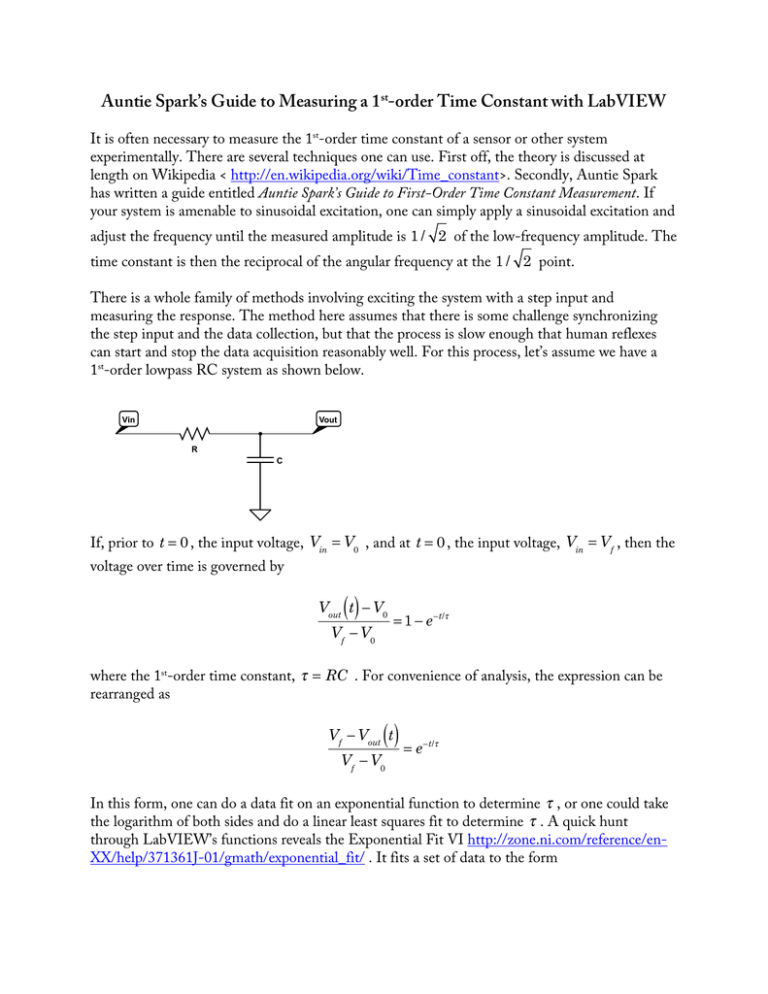
Auntie Spark’s Guide to Measuring a 1st-order Time Constant with LabVIEW
It is often necessary to measure the 1st-order time constant of a sensor or other system
experimentally. There are several techniques one can use. First off, the theory is discussed at
length on Wikipedia < http://en.wikipedia.org/wiki/Time_constant>. Secondly, Auntie Spark
has written a guide entitled Auntie Spark’s Guide to First-Order Time Constant Measurement. If
your system is amenable to sinusoidal excitation, one can simply apply a sinusoidal excitation and
adjust the frequency until the measured amplitude is 1 / 2 of the low-frequency amplitude. The
time constant is then the reciprocal of the angular frequency at the 1 / 2 point.
There is a whole family of methods involving exciting the system with a step input and
measuring the response. The method here assumes that there is some challenge synchronizing
the step input and the data collection, but that the process is slow enough that human reflexes
can start and stop the data acquisition reasonably well. For this process, let’s assume we have a
1st-order lowpass RC system as shown below.
Vin
Vout
R
C
If, prior to t = 0 , the input voltage, Vin = V0 , and at t = 0 , the input voltage, Vin = Vf , then the
voltage over time is governed by
()
Vout t − V0
Vf − V0
= 1 − e −t/τ
where the 1st-order time constant, τ = RC . For convenience of analysis, the expression can be
rearranged as
( )=e
Vf − Vout t
−t/τ
Vf − V0
In this form, one can do a data fit on an exponential function to determine τ , or one could take
the logarithm of both sides and do a linear least squares fit to determine τ . A quick hunt
through LabVIEW’s functions reveals the Exponential Fit VI http://zone.ni.com/reference/enXX/help/371361J-01/gmath/exponential_fit/ . It fits a set of data to the form
y = aebx + c
where a is the amplitude, b is the damping, and c is the offset. With a little rearrangement to
() (
)
Vout t = V0 − Vf e −t/τ + Vf
one can readily see that a = V0 − Vf , b = −1 / τ , and c = Vf . What we need is a VI that will let
us sample a waveform until we have a full section of step response, and will let us trim the
collected data down to just the step response, and then let us fit our data, and we can calculate τ
as −1 / b .
Let’s use our VI and DAQ to measure the time constant of a 390 kΩ resistor in series with a
0.68 µF capacitor. The time constant should be roughly 390 ×103 i 0.68 ×10−6 = 0.265 s . We’ll
need to wait about six time constants to get a good response and 12 to make sure, or 24 time
constants if we’re putting in a square wave, so the signal frequency should be about
f=
1
= 0.157 Hz ≈ 1.5 Hz
24 i 0.265 s
to get decent signals to process. The signal generator is connected between Vin and GND and the
output is measured between Vout and GND. Both the input and output are measured with a
myDAQ with the input on AI0 and the output on AI1. The instructions for connecting a myDAQ
can be found elsewhere.
Conceptually, we want to start the acquisition, look at each buffer, concatenate the buffers
together, look at the concatenated buffers, and stop when the signal is long enough and has a
clean rise and decay or fall and decay.
To get contiguous buffers, we want to use the DAQ Assistant and set it to Continuous Samples.
We want both analog input channels so we’ve selected both ai0 and ai1 on the myDAQ.
To make following signals easier we’ve renamed them as Input and Output. To make the later
calculations easier, we’ve set the sample rate to 1000 SPS and the samples per buffer (Samples
to Read) to 100. 100 samples at 1000 SPS means that the buffer will take 0.1 seconds to fill.
If you set the DAQ Assistant to Continuous Samples and click OK, it will ask if you want the
DAQ Assistant in a while loop (if it’s not already in one). You want it in one. You’ll want to
stretch out the loop to make more room for other subVIs.
Getting the VI to display the contents of each buffer when it fills (every 0.1 seconds of our signal
in this case) is easy. Just right-click on the Data output of the DAQ Assistant and Create ->
Graph Indicator. At this point, save and run your VI to see if the signal updates every 0.1
seconds as expected.
The question arises as to how to concatenate all of the individual buffers together. The Signal
Manipulation pallet under the Express VI pallet has a VI called Append Signals.
It will append a signal on the end of another signal. If we somehow had all of the previous
signals concatenated together we could add the new signal at the end. Inside the VI there is a
checkbox for Append only if t0 aligns and dt matches. When checked, the VI will only append
the new signal if it has the same Δt as the old signal and its start time is one sample period after
the last sample in the old signal. You should make sure the checkbox is checked.
It will make sure your concatenated signal is contiguous. The best way to pass the concatenated
signal from one loop to the next is with a shift register. However, on the first loop you need to
start with the first buffer, not append the buffer to the previous signal. We’ll handle the startup
with a case structure and a conditional. We’ll see if the loop counter equals zero. If so, simply
pass on the first buffer to the shift register.
If not, append the new buffer to the previous buffers. The resultant loop is shown below.
Don’t forget to add a second Graph Indicator at the output of the case structure. This graph
should show you the complete concatenated waveform.
Save and Run your VI. The Buffer Display should update every 0.1 seconds and the
Concatenated Display should show you the complete waveform. When you have a full rise or fall
from your waveform click the STOP button and the VI will quit collecting data.
Great! We can now watch our data and stop it when we have what we want, but the graph
indicators don’t help us calculate the time constant much (Actually, you can print out the full
waveform and either determine when the step response has made it 63% of the way to its final
value, or draw the tangent to the initial part of the curve and see where it hits the final value line
as ways to determine the time constant). We’d like to be able to select a portion of the final curve
and use the Exponential Fit VI to determine the time constant. Since we’ll probably want to
adjust the selected portion until we get what we want, let’s put the selection process inside of a
while loop. If you select the while loop from the Express pallet, it will automatically create the
STOP button. Otherwise, you have to add the STOP button manually.
The Express VI to extract a portion of a signal is called Extract Portion of Signal (Express ->
Signal Manipulation).
Inside there are several selection possibilities. For a quick and simple VI it’s probably best to
choose Begin at Sample Number and Number of Samples.
It’s easy to guess and enter a starting sample and number of samples, but it’s much harder to
enter a starting time stamp, which is why we don’t choose “Begin at offset” or “Length”.
However, you can certainly select them and experiment if you wish. After clicking OK the VI
should appear and have connection spots for Begin Sample and Samples. Right click on them
and create controls for both. If you want to get fancy you can replace the controls with dials or
sliders, but again for a quick VI numeric controls are easiest.
The remaining parts of the loop are to get the signal in the correct format for the Exponential Fit
VI and to get good range limits for the fit. The VI in region 1 in the figure below splits the two
channels (input and output) into separate channels and we only want to process the output. The
pieces in region 2 convert the dynamic signal into a waveform and then extract the Δt and array
of values from the waveform. The For Loop at region 3 generates an array of time values starting
at 0 of the same length as the value array. The fitting algorithm in region 7 works best if given
reasonable ranges for the fitted parameters. The VIs in region 4 essentially determine the
magnitude of the max value minus the min value and multiply by two to give limits for the
amplitude, a , above. The objects in regions 5 and 6 are created in the following manner: Right
click on the Parameter Bounds terminal of the Exponential Fit VI and create a constant. Right
click on the brown wire and insert a Bundle by Name from the Cluster, … pallet. Then drag the
bottom edge of the newly created object to expand it by one slot. If you want, you can expand it
to six spaces and see the name of each input element in the cluster. You could also set the values
that way. Any that you don’t set with the Bundle by Name use the default value from the cluster.
As explained above, the range for the amplitude is determined from the data. The next two
values are the range for the damping. Since the damping, b , is assumed to be negative, we’ve set
the range to be between −∞ and 0. The final two values are for the offset. We could narrow the
range a bit by choosing limiting values, but –Inf (for −∞ ) and Inf work well enough. With the
remaining indicators and subVIs set up, we’re ready to test out the VI. Here is the VI after
having run for about 4 seconds.
After about 13.5 seconds we seem to have enough data so we click on the Stop Collecting Data
button.
We’ll now try to fit the 1st-order rise that occurs at about 7 seconds. 7 seconds at 1000 SPS is
7000 sample, so we’ll try 6800 (just under 7000) in the Start with Sample # box, and process 2
seconds or 2000 samples of data.
The fit isn’t bad, but we should get closer to the start of the step change, so we’ll guess 6900 as
the starting sample. We got closer to the step, but we still caught a little of the pre-step.
We’ll make a guess of 6950 for the starting sample. In this case we miss all of the pre-step. The
time constant appears to be 0.2935 s, which is very close to our calculated value of 0.265 s from
the nominal part values. The fit is so good, we can’t tell the fitted curve from the data points.
To double check, let’s start at the falling signal at about 2.5 s. Our first guess will be 2800. It’s a
bit early. So let’s try something a little later.
Our second guess is 3000 and still has a little of the pre-step in it. Let’s go one more guess.
The third guess is 3050 and it seems to miss all of the pre-step. The fit gives us a time constant of
0.2937 s, which is very close to the earlier value of 0.2935 s.
Were we interested in doing some reasonable statistics, we could repeat the data collection and
fitting, and then use our Students t-test table and the mean and standard deviation of our fit time
constants to give us the time constant with the experimental uncertainty.