CS281B / Stat 241B : Statistical Learning Theory
Lecture: #22 on 19 Apr 2004
Dirichlet Process I
Lecturer: Prof. Michael Jordan
22.1
Scribe: Daniel Schonberg dschonbe@eecs.berkeley.edu
Dirichlet Distribution
The Dirichlet distribution was introduced in the last lecture. Posterior inference under a Dirichlet prior will
be summarized here.
δ
δ
δ
α
1
(a)
δ
α
α
2
3
δ
δ
α
n
(b)
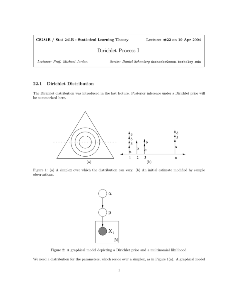
Figure 1: (a) A simplex over which the distribution can vary. (b) An initial estimate modified by sample
observations.
α
p
Xi
Ν
Figure 2: A graphical model depicting a Dirichlet prior and a multinomial likelihood.
We need a distribution for the parameters, which reside over a simplex, as in Figure 1(a). A graphical model
1
2
Dirichlet Process I
is shown in Figure 2. The estimate is based upon the prior distribution and the effects of the observed data
as in Figure 1(b)
p(p1 , . . . , pk |x1 , . . . , xn ) ∼ Dir(α1 +
n
X
δ1 (xi ), . . . , αk +
n
X
δk (xi )
(1)
i=1
i=1
=
X
αj
1
+
δj (xi )
α+ + n α+ + n i=1
(2)
=
n
1X
αj α+
+
δj (xi )
α+ α+ + n α+ + n n i=1
(3)
n
p(xn+1 = j|x1 , . . . , xn , α1 , . . . , αn )
n
where α+ =
Pn
i=1
αi .
We can compute the expected value of the pi ’s as E[pi ] = αi /α+ .
This model is related to the Polya Urn Model. In that model, we take one ball out of a bin, we then put
that ball and another one of the same color back in the bin.
22.2
Dirichlet Process - View 1
In this view of the Dirichlet Process, we begin with any probability measure G 0 on the reals. The values for
each of the partitions β is given according to this measure as suggested in Figure 3.
G0
β
1
β
2
β
3
β4
β5
....
β
K
Figure 3: Here, G0 can be any probability measure. The various β values are determined by the measure in
the corresponding region.
A process is a Dirichlet process if the following equation holds for all partitions:
(p(β1 ), . . . , p(βk )) ∼ Dir(αG0 (β1 ), αG0 (β2 ), . . . , αG0 (βk ))
(4)
We denote a sample from the Dirichlet process as G ∼ DP (α, G0 ), where α is a concentration parameter
and G0 is the base probability measure (see Figure 4).
Some properties are as follows.
• E[G] = G0 . This is analogous to the fact that E[pi ] = αi /α+ .
Pn
1
α
G0 + α+n
• p(G|θ1 , . . . , θn ) = DP (α + n, α+n
i=1 δθi ). This effect of the θ’s on the distribution of G is
suggested in Figure 5.
3
Dirichlet Process I
α
G0
G
θi
Figure 4: The graphical model for a Dirichlet Process generating the θ parameters.
{θ i }
Figure 5: An example of how the observed values will change the distribution estimate.
• E[G|θ1 , . . . , θn ] =
α
α+n G0
+
1
α+n
Pn
i=1 δi
We now examine the marginal probabilities for a new θ.
1 X
= θi for 1 ≤ i ≤ n|θ1 , . . . , θn , α, G0 ) =
δθ (θn+1 )
α + n j=1 j
n
p(θn+1
p(θn+1 6= θi for 1 ≤ i ≤ n|θ1 , . . . θn , α, G0 ) =
α
α+n
(5)
(6)
These conditionals can be interpreted in terms of the so-called Chinese restaurant process. In this process,
a restaurant possesses a countably infinite collection of empty tables. As customers arrive, they can either
sit at a new table or join someone else’s table. An example is shown in Figure 6.
x
x
x
x
x
x
x
x
....
x
Figure 6: A diagram of the Chinese restaurant process. In this process, people arrive and are seated at
tables. They either sit at a new table or join an already occupied table.
Suppose for example that α = 1 and n = 1. The first customer occupies the first table. The next customer
will either start a new table with probability 1/2 or join the first table with probability 1/2. After N
4
Dirichlet Process I
customers have arrived, the number of occupied tables is random and grows as O(log N ). There is an
isomorphism between the tables and the cycle structure of random permutations.
It turns out that the specific ordering of the customers is irrelevant; i.e., the Chinese restaurant process
yields an exchangeable distribution on partitions of the integers.
Recall that an infinite set of random variables is said to be infinitely exchangeable if for every finite subset
{x1 , x2 , . . . , xn } we have
p(x1 , x2 , . . . , xn ) = p(xπ(1) , xπ(2) , . . . , xπ(n) )
for any permutation π.
Theorem 1 (De Finetti) A set of random variables is infinitely exchangeable if and only if
p(x1 , . . . , xn ) =
Z Y
n
p(xi |θ)dP (θ)
(7)
i=1
for some θ and some measure P (θ).
In particular, one possible choice for P (θ) is the Dirichlet process (where the preferred notion is “G” instead
of “θ”).
22.3
Dirichlet Process - View 2
The second representation we consider is the stick-breaking view. This representation gives a more concrete
meaning to “G ∼ DP (α, G0 ).”
Figure 7: A sample measure and the resulting discrete Dirichlet Process.
It turns out that there is an explicit representation for samples G from the Dirichlet process. This representation is as follows:
∞
X
G=
(8)
πk δ θ k
k=1
In this equation, both the πk and the θk are random. The πk are distributed as follows:
πk = πk0
k−1
Y
(1 − πl ),
l=1
where πk0 ∼ Beta(1, α). The θk are distributed as θk ∼ G0 .
A diagram of the stick-breaking process is shown in Figure 8.
(9)
5
Dirichlet Process I
π1
π2
π3
0
(1− π1) (1− π2)
1
(1− π1)
Figure 8: A diagram of the stick-breaking interpretation of the Dirichlet Process.
From Figure 8, we can obtain that π1 = π10 , π2 = π20 (1 − π1 ), and so on.
In the next lecture we will consider using Dirichlet processes in the context of mixture models (see Figure 9).
The basic interpretation is that G is a generator of atoms that serve as parameters of mixture components
in a mixture model.
α
G0
G
θi
Xi
N
Figure 9: The graphical model for the Dirichlet Process mixture model..