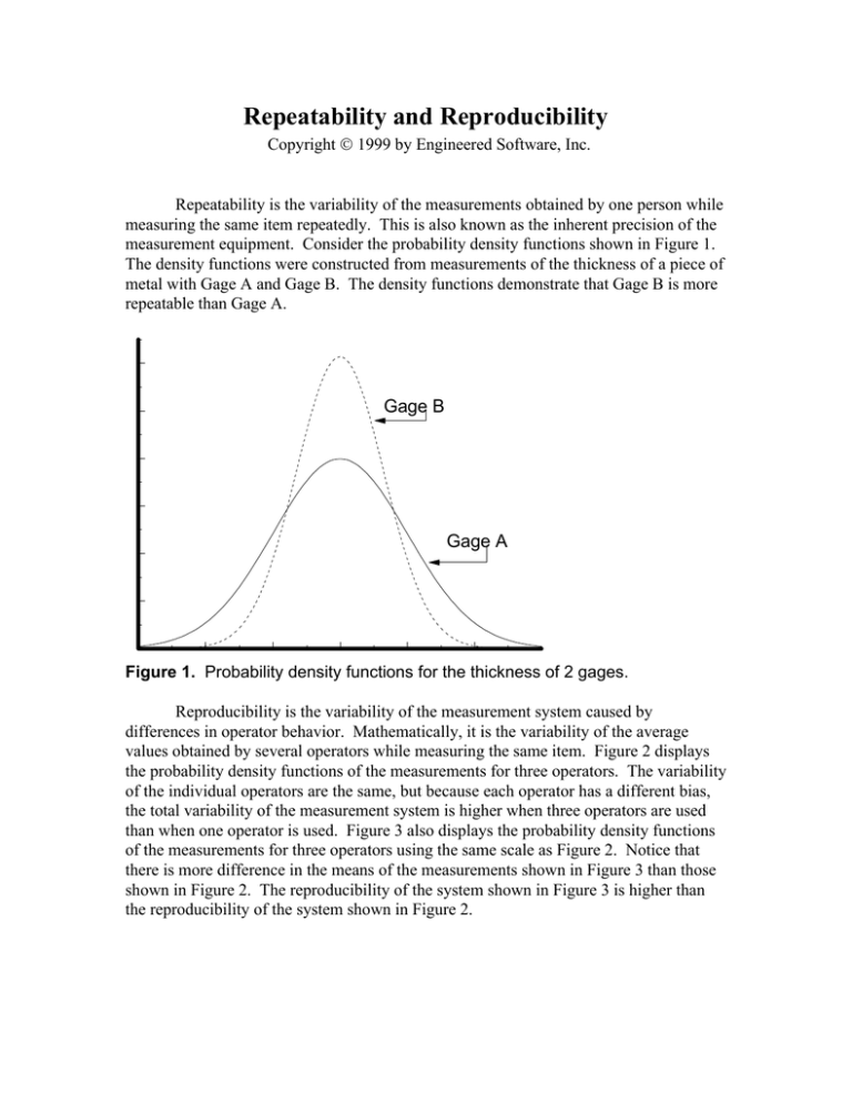
Repeatability and Reproducibility
Copyright  1999 by Engineered Software, Inc.
Repeatability is the variability of the measurements obtained by one person while
measuring the same item repeatedly. This is also known as the inherent precision of the
measurement equipment. Consider the probability density functions shown in Figure 1.
The density functions were constructed from measurements of the thickness of a piece of
metal with Gage A and Gage B. The density functions demonstrate that Gage B is more
repeatable than Gage A.
Gage B
Gage A
Figure 1. Probability density functions for the thickness of 2 gages.
Reproducibility is the variability of the measurement system caused by
differences in operator behavior. Mathematically, it is the variability of the average
values obtained by several operators while measuring the same item. Figure 2 displays
the probability density functions of the measurements for three operators. The variability
of the individual operators are the same, but because each operator has a different bias,
the total variability of the measurement system is higher when three operators are used
than when one operator is used. Figure 3 also displays the probability density functions
of the measurements for three operators using the same scale as Figure 2. Notice that
there is more difference in the means of the measurements shown in Figure 3 than those
shown in Figure 2. The reproducibility of the system shown in Figure 3 is higher than
the reproducibility of the system shown in Figure 2.
Figure 2. Reproducibility demonstration.
Figure 3. Reproducibility demonstration.
The most commonly used method for computing repeatability and reproducibility
is the Range and Average method. The ANOVA method is more accurate, but because
of the complex mathematics involved it has been shunned historically. With desktop
computers there is no excuse for not using the more accurate ANOVA method.
Range & Average Method
The Range & Average Method computes the total measurement system
variability, and allows the total measurement system variability to be separated into
repeatability, reproducibility, and part variation.
The ANOVA method, discussed in the next section, is preferred to the average
range method. The ANOVA method quantifies the interaction between repeatability and
reproducibility, and is considered to be more accurate than the average and range
method.
To quantify repeatability and reproducibility using average and range method,
multiple parts, appraisers, and trials are required. The recommended method is to use 10
parts, 3 appraisers and 2 trials, for a total of 60 measurements. The measurement system
repeatability is
Repeatability =
. R
515
d2
1
where R is the average of the ranges for all appraisers and parts, and
d2 is found in Appendix A with Z = the number of parts times the number of
appraisers, and W = the number of trials.
The measurement system reproducibility is
2
 5.15X range 
Repeatability 2
 −
Reproducibility = 
nr
d2


2
where X range is the average of the difference in the average measurements between the
appraiser with the highest average measurements, and the appraiser with the
lowest average measurements, for all appraisers and parts,
d2 is found in Appendix A with Z = 1 and W = the number of appraisers,
n is the number of parts, and
r is the number of trials.
The measurement system repeatability and reproducibility is
R& R = Repeatability 2 + Reproducibility 2
3
The part variability is
VP =
515
. RP
d2
4
where Rp is the difference between the largest average part measurement and the smallest
average part measurement, where the average is taken for all appraisers and all
trials, and
d2 is found in Appendix A with Z = 1 and W = the number of parts.
The total variability, measurement system variability and part variation combined is
VT =
R& R 2 + V P2
5
Example 1
The thickness, in millimeters, of 10 parts have been measured by 3 operators, using the
same measurement equipment. Each operator measured each part twice, and the data is
given in Table 1.
Table 1. Range & Average method example data.
Operator
A
B
C
Part
Trial 1
Trial 2
Trial 1
Trial 2
Trial 1
Trial 2
1 65.2 60.1 62.9 56.3 71.6 60.6
2 85.8 86.3 85.7 80.5 92.0 87.4
3 100.2 94.8 100.1 94.5 107.3 104.4
4 85.0 95.1 84.8 90.3 92.3 94.6
5 54.7 65.8 51.7 60.0 58.9 67.2
6 98.7 90.2 92.7 87.2 98.9 93.5
7 94.5 94.5 91.0 93.4 95.4 103.3
8 87.2 82.4 83.9 78.8 93.0 85.8
9 82.4 82.2 80.7 80.3 87.9 88.1
10 100.2 104.9 99.7 103.2 104.3 111.5
Repeatability is computed using the average of the ranges for all appraiser and all
parts. This data is given in Table 2.
Table 2. Example problem range calculations.
Operator
A
B
Part Trial 1 Trial 2 R
C
Trial 1 Trial 2 R Trial 1 Trial 2 R
1
65.2
60.1
5.1
62.9
56.3
6.6
71.6
60.6 11.0
2
85.8
86.3
0.5
85.7
80.5
5.2
92.0
87.4
3
100.2
94.8
5.4 100.1
94.5
5.6 107.3 104.4 2.9
4
85.0
95.1 10.1 84.8
90.3
5.5
5
54.7
65.8 11.1 51.7
60.0
8.3
58.9
67.2
8.3
6
98.7
90.2
8.5
92.7
87.2
5.5
98.9
93.5
5.4
7
94.5
94.5
0.0
91.0
93.4
2.4
95.4
103.3 7.9
8
87.2
82.4
4.8
83.9
78.8
5.1
93.0
85.8
7.2
9
82.4
82.2
0.2
80.7
80.3
0.4
87.9
88.1
0.2
10
100.2 104.9 4.7
99.7
103.2 3.5 104.3 111.5 7.2
92.3
94.6
4.6
2.3
The average of the 30 ranges, R , is 5.20. From Appendix A, with Z = 30 (10 parts
multiplied by 3 appraisers) and W = 2 (2 trials), d2 is 1.128. The repeatability is
Repeatability =
. (5.20)
515
= 23.7
1128
.
The average reading for appraiser A is 85.5, the average reading for appraiser B is 82.9,
and the average reading for appraiser C is 88.9. To compute reproducibility, the average
of the range between the appraiser with the smallest average reading (appraiser B in this
example) and the appraiser with the largest average reading (appraiser C in this example)
is needed. Table 3 shows this data.
Table 3. Reproducibility example computations.
Part
1
2
3
4
5
6
7
8
9
10
1
2
3
4
5
6
7
8
9
10
Trial
1
1
1
1
1
1
1
1
1
1
2
2
2
2
2
2
2
2
2
2
Operator B
62.9
85.7
100.1
84.8
51.7
92.7
91.0
83.9
80.7
99.7
56.3
80.5
94.5
90.3
60.0
87.2
93.4
78.8
80.3
103.2
Operator C
71.6
92.0
107.3
92.3
58.9
98.9
95.4
93.0
87.9
104.3
60.6
87.4
104.4
94.6
67.2
93.5
103.3
85.8
88.1
111.5
R
8.7
6.3
7.2
7.5
7.2
6.2
4.4
9.1
7.2
4.6
4.3
6.9
9.9
4.3
7.2
6.3
9.9
7.0
7.8
8.3
The average of the ranges, X range , is 7.015. From Appendix A, using Z = 1 and W = 3
for 3 appraisers, is 1.91. The reproducibility is
 515
. ( 7.015) 
23.7 2
= 18.2
Reproducibility = 
 −


.
191
10(2)
2
The repeatability and reproducibility is
R & R = 23.7 2 + 18.2 2 = 29.9
The part variability is computed using the difference between the largest and smallest
part measurement, where the average is taken for all parts and appraisers. This data is
shown in Table 4.
Table 4. Example part variability computations.
Operator
A
Part
B
C
Trial 1 Trial 2 Trial 1 Trial 2 Trial 1 Trial 2
Avg
1
65.2
60.1
62.9
56.3
71.6
60.6
2
85.8
86.3
85.7
80.5
92.0
87.4
62.78
86.28
3
100.2
94.8
100.1
94.5
107.3
104.4
100.22
4
85.0
95.1
84.8
90.3
92.3
94.6
90.35
5
54.7
65.8
51.7
60.0
58.9
67.2
59.72
6
98.7
90.2
92.7
87.2
98.9
93.5
93.53
7
94.5
94.5
91.0
93.4
95.4
103.3
95.35
8
87.2
82.4
83.9
78.8
93.0
85.8
85.18
9
82.4
82.2
80.7
80.3
87.9
88.1
83.60
10
100.2
104.9
99.7
103.2
104.3
111.5
103.97
The part with the largest average belongs to part 10, 103.97. The lowest average belongs
to part 5, 59.72. This difference , 44.25, is Vp. From Appendix A, using Z = 1 and W =
10 for 10 parts, d2 = 3.18. The part variability is
VP =
515
. ( 44.25)
= 717
.
318
.
The total measurement system variability is
VT = 29.9 2 + 717
. 2 = 77.7
Analysis of Variance Method
The analysis of variance method (ANOVA) is the most accurate method for
quantifying repeatability and reproducibility. In addition, the ANOVA method allows
the variability of the interaction between the appraisers and the parts to be determined.
The ANOVA method for measurement assurance is the same statistical technique
used to analyze the effects of different factors in designed experiments. The ANOVA
design used is a two-way, fixed effects model with replications. The ANOVA table is
shown in Table 5.
Table 5. Two-Way ANOVA Table.
Source of
Variation
Appraiser
Sum of
Square
s
SSA
Degrees
of
Freedom
a-1
Parts
SSB
b-1
Interaction
(Appraiser,
Parts)
Gage
(Error)
SSAB
(a-1)(b-1)
MSAB =
SSE
ab(n-1)
MSE =
Total
TSS
N-1
Mean
Square
SSA
a −1
SSB
MSB =
b −1
MSA =
SSAB
(a − 1)(b − 1)
F Statistic
F=
MSA
MSE
F=
MSB
MSE
F =
M SA B
M SE
SSE
ab(n − 1)
(Yi .. ) 2 Y••2
−
SSA = ∑
bn
N
i =1
2
b (Y )
Y••2
. j.
−
SSB = ∑
an
N
j =1
a
a
b
SSAB = ∑ ∑
i =1 j =1
a
b
(Yij . ) 2
n
−
6
7
Y••2
− SSA − SSB
N
n
TSS = ∑ ∑ ∑ Yijk2 −
i =1 j =1 k =1
Y••2
N
SSE = TSS − SSA − SSB − SSAB
8
9
10
a = number of appraisers,
b = number parts,
n = the number of trials, and
N = total number of readings (abn)
When conducting a study, the recommended procedure is to use 10 parts, 3
appraisers and 2 trials, for a total of 60 measurements. The measurement system
repeatability is
Repeatability = 515
.
MSE
11
The measurement system reproducibility is
.
Reproducibility = 515
MSA − MSAB
bn
12
The interaction between the appraisers and the parts is
MSAB − MSE
n
I = 515
.
13
The measurement system repeatability and repeatability is
R & R = Repeatability 2 + Reproducibility 2 + I 2
14
The measurement system part variation is
V P = 515
.
MSB − MSAB
an
15
The total measurement system variation is
VT =
R& R 2 + V P2
16
Example 2
The thickness, in millimeters, of 10 parts have been measured by 3 operators, using the
same measurement equipment. Each operator measured each part twice, and the data is
given in Table 6.
Table 6. ANOVA method example data.
Operator
A
B
C
Part Trial 1 Trial 2 Trial 1 Trial 2 Trial 1 Trial 2
1
65.2
60.1
62.9
56.3
2
85.8
3
100.2
4
5
71.6
60.6
86.3
85.7
80.5
92.0
87.4
94.8
100.1
94.5
107.3
104.4
85.0
95.1
84.8
90.3
92.3
94.6
54.7
65.8
51.7
60.0
58.9
67.2
6
98.7
90.2
92.7
87.2
98.9
93.5
7
94.5
94.5
91.0
93.4
95.4
103.3
8
87.2
82.4
83.9
78.8
93.0
85.8
9
82.4
82.2
80.7
80.3
87.9
88.1
10
100.2
104.9
99.7
103.2
104.3
111.5
To compute the characteristics of this measurement system, the two-way
ANOVA table must be completed. The sum of the 20 readings (10 parts multiplied by 2
trials) for appraiser A is 1710.2. The sum of the 20 readings for appraiser B is 1657.7.
The sum of the 20 readings for appraiser C is 1798.0, and the sum of all 60 readings is
5165.9. The sum-of-squares for the appraisers is
SSA =
1710.2 2 1657.7 2 1798.0 2 5165.9 2
+
+
−
= 502.5
10(2)
10(2)
10(2)
60
The sum of the 6 readings for each part (3 appraisers multiplied by 2 trials) is given in
Table 7 along with the square of this sum, and the square of this sum divided by 6.
Table 7. Part sum-of-squares computations.
Part
1
2
3
4
5
6
7
8
9
10
Total
Sum
376.7
517.7
601.3
542.1
358.3
561.2
572.1
511.1
501.6
623.8
Sum Squared
Sum Squared/6
141,902.9
268,013.3
361,561.7
293,872.4
128,378.9
314,945.4
327,298.4
261,223.2
251,602.6
389,126.4
23,650.5
44,668.9
60,260.3
48,978.7
21,396.5
52,490.9
54,549.7
43,537.2
41,933.8
64,854.4
456,320.9
The sum-of-squares for the parts is
SSB = 456,320.9 −
5165.9 2
= 11,5455
.
60
The sum of the 2 trials for each combination of appraiser and part is given in Table 8
along with the square of this sum, and the square of this sum divided by 2.
Table 8. Interaction sum-of-square computations.
Part
1
2
3
4
5
6
7
8
9
10
1
2
3
4
5
6
7
8
9
10
1
2
3
4
5
6
7
8
9
10
Total
Appraiser
A
A
A
A
A
A
A
A
A
A
B
B
B
B
B
B
B
B
B
B
C
C
C
C
C
C
C
C
C
C
Sum
125.3
172.1
195.0
180.1
120.5
188.9
189.0
169.6
164.6
205.1
119.2
166.2
194.6
175.1
111.7
179.9
184.4
162.7
161.0
202.9
132.2
179.4
211.7
186.9
126.1
192.4
198.7
178.8
176.0
215.8
Sum Squared
15,700.1
29,618.4
38,025.0
32,436.0
14,520.3
35,683.2
35,721.0
28,764.2
27,093.2
42,066.0
14,208.6
27,622.4
37,869.2
30,660.0
12,476.9
32,364.0
34,003.4
26,471.3
25,921.0
41,168.4
17,476.8
32,184.4
44,816.9
34,931.6
15,901.2
37,017.8
39,481.7
31,969.4
30,976.0
46,569.6
Sum Squared/2
7,850.0
14,809.2
19,012.5
16,218.0
7,260.1
17,841.6
17,860.5
14,382.1
13,546.6
21,033.0
7,104.3
13,811.2
18,934.6
15,330.0
6,238.4
16,182.0
17,001.7
13,235.6
12,960.5
20,584.2
8,738.4
16,092.2
22,408.4
17,465.8
7,950.6
18,508.9
19,740.8
15,984.7
15,488.0
23,284.8
456,859.0
The sum-of-squares for the interaction between the appraisers and the parts, SSAB, is
5165.9 2
SSAB = 456,859.0 −
− 502.5 − 11,545.5 = 35.6
60
Squaring all 60 individual reading and summing the values gives 457,405.8. The total
sum-of-squares is
TSS = 457,4058
. −
5165.9 2
= 12,630.4
60
The sum-of-squares for the gage or error is
SSE = 12,630.4 − 502.5 − 11,5455
. − 35.6 = 546.8
There are 2 degrees-of-freedom for the appraisers, the number of appraisers
minus one; 9 degrees-of-freedom for the parts, the number of parts minus one, 18
degrees-of-freedom for the interaction between the appraisers and the parts, the number
of appraisers minus one multiplied by the number of parts minus one; 59 total degreesof-freedom; the total number of readings minus one, and 30 degrees-of-freedom for the
gage, total degrees-of-freedom minus the degrees-of-freedom for the appraisers minus the
degrees-of-freedom for the parts minus the degrees-of-freedom for the interaction. Since
the mean-square-error is the sum-of-square divided by the degrees-of-freedom, the
ANOVA table can be completed as shown in Table 9.
Table 9. Example ANOVA table.
Source of
Variation
Appraiser
Degrees
Sum of
of
Mean
Squares Freedom Square
502.5
2
251.3
13.8
Significance
0.000057
Parts
11,545.5
9
1,282.8
70.4
0.000000
35.6
18
1.98
0.11
0.999996
Interaction
(Appraisers,
Parts)
Gage (Error)
Total
546.8
30
18.2
12,630.4
59
214.1
F
The significance listed in Table 9 represents the probability of Type I error.
Stated another way, if the statement is made “the appraisers are a significant source of
measurement variability”, the probability of this statement being incorrect is 0.000057.
This significance is the area under the F probability density function to the right of the
computed F-statistic. This value can be found using the function FDIST(F-statistic,d1,d2)
in Microsoft Excel or Lotus 123, where d1 and d2 are the appropriate degrees of freedom.
Continuing with the example, the repeatability is
Repeatability = 515
. 18.2 = 22.0
Reproducibility is
Reproducibility = 515
.
2513
. − 198
.
= 18.2
10( 2)
The interaction between the appraisers and the parts is
I = 515
.
198
. − 18.2
= cannot be computed
n
Obviously the variability due to the interaction cannot be imaginary (the square root of a
negative number is an imaginary number); what happened? Each mean square is an
estimate subject to sampling error. In some cases the estimated variance will be negative
or imaginary. In these cases, the estimated variance is zero.
The repeatability and reproducibility is
R & R = 22 2 + 18.2 2 + 0 2 = 28.6
The part variation is
.
V P = 515
1,282.8 − 198
.
= 75.2
3( 2)
The total measurement system variation is
VT = 28.6 2 + 75.2 2 = 80.5
Appendix A - Values of d2
z
1
2
3
4
5
6
7
8
9
10
11
12
13
14
15
>15
2
1.41
1.28
1.23
1.21
1.19
1.18
1.17
1.17
1.16
1.16
1.15
1.15
1.15
1.15
1.15
1.128
3
1.91
1.81
1.77
1.75
1.74
1.73
1.73
1.72
1.72
1.72
1.71
1.71
1.71
1.71
1.71
1.693
4
2.24
2.15
2.12
2.11
2.10
2.09
2.09
2.08
2.08
2.08
2.08
2.07
2.07
2.07
2.07
2.059
5
2.48
2.40
2.38
2.37
2.36
2.35
2.35
2.35
2.34
2.34
2.34
2.34
2.34
2.34
2.34
2.326
6
2.67
2.60
2.58
2.57
2.56
2.56
2.55
2.55
2.55
2.55
2.55
2.55
2.55
2.54
2.54
2.534
7
2.83
2.77
2.75
2.74
2.78
2.73
2.72
2.72
2.72
2.72
2.72
2.72
2.71
2.71
2.71
2.704
w
8
2.96
2.91
2.89
2.88
2.87
2.87
2.87
2.87
2.86
2.86
2.86
2.85
2.85
2.85
2.85
2.847
9
3.08
3.02
3.01
3.00
2.99
2.99
2.99
2.98
2.98
2.98
2.98
2.98
2.98
2.98
2.98
2.97
10
3.18
3.13
3.11
3.10
3.10
3.10
3.10
3.09
3.09
3.09
3.09
3.09
3.09
3.09
3.08
3.078
11
3.27
3.22
3.21
3.20
3.19
3.19
3.19
3.19
3.19
3.18
3.18
3.18
3.18
3.18
3.18
3.173
12
3.35
3.30
3.29
3.28
3.28
3.27
3.27
3.27
3.27
3.27
3.27
3.27
3.27
3.27
3.26
3.258
13
3.42
3.38
3.37
3.36
3.36
3.35
3.35
3.35
3.35
3.34
3.34
3.34
3.34
3.34
3.34
3.336
14
3.49
3.45
3.43
3.43
3.42
3.42
3.42
3.42
3.42
3.42
3.41
3.41
3.41
3.41
3.41
3.407
15
3.55
3.51
3.50
3.49
3.49
3.49
3.48
3.48
3.48
3.48
3.48
3.48
3.48
3.48
3.48
3.472