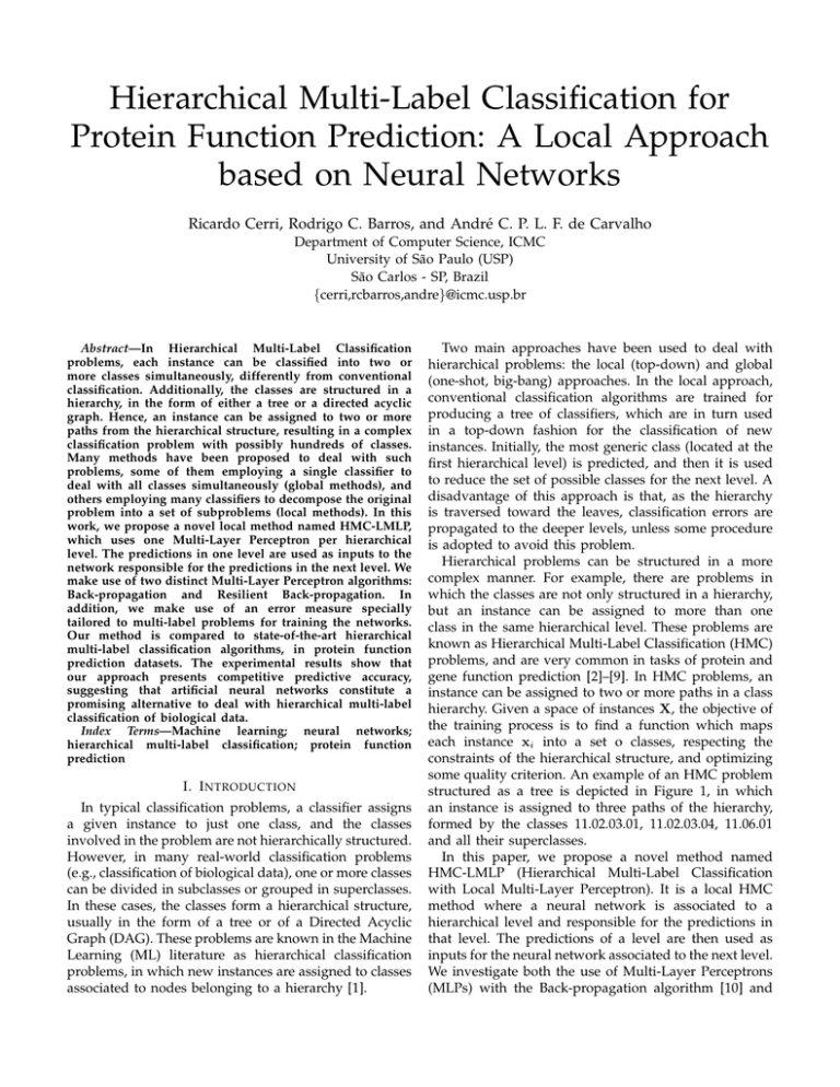
Hierarchical Multi-Label Classification for
Protein Function Prediction: A Local Approach
based on Neural Networks
Ricardo Cerri, Rodrigo C. Barros, and André C. P. L. F. de Carvalho
Department of Computer Science, ICMC
University of São Paulo (USP)
São Carlos - SP, Brazil
{cerri,rcbarros,andre}@icmc.usp.br
Abstract—In Hierarchical Multi-Label Classification
problems, each instance can be classified into two or
more classes simultaneously, differently from conventional
classification. Additionally, the classes are structured in a
hierarchy, in the form of either a tree or a directed acyclic
graph. Hence, an instance can be assigned to two or more
paths from the hierarchical structure, resulting in a complex
classification problem with possibly hundreds of classes.
Many methods have been proposed to deal with such
problems, some of them employing a single classifier to
deal with all classes simultaneously (global methods), and
others employing many classifiers to decompose the original
problem into a set of subproblems (local methods). In this
work, we propose a novel local method named HMC-LMLP,
which uses one Multi-Layer Perceptron per hierarchical
level. The predictions in one level are used as inputs to the
network responsible for the predictions in the next level. We
make use of two distinct Multi-Layer Perceptron algorithms:
Back-propagation and Resilient Back-propagation. In
addition, we make use of an error measure specially
tailored to multi-label problems for training the networks.
Our method is compared to state-of-the-art hierarchical
multi-label classification algorithms, in protein function
prediction datasets. The experimental results show that
our approach presents competitive predictive accuracy,
suggesting that artificial neural networks constitute a
promising alternative to deal with hierarchical multi-label
classification of biological data.
Index Terms—Machine learning; neural networks;
hierarchical multi-label classification; protein function
prediction
I. I NTRODUCTION
In typical classification problems, a classifier assigns
a given instance to just one class, and the classes
involved in the problem are not hierarchically structured.
However, in many real-world classification problems
(e.g., classification of biological data), one or more classes
can be divided in subclasses or grouped in superclasses.
In these cases, the classes form a hierarchical structure,
usually in the form of a tree or of a Directed Acyclic
Graph (DAG). These problems are known in the Machine
Learning (ML) literature as hierarchical classification
problems, in which new instances are assigned to classes
associated to nodes belonging to a hierarchy [1].
Two main approaches have been used to deal with
hierarchical problems: the local (top-down) and global
(one-shot, big-bang) approaches. In the local approach,
conventional classification algorithms are trained for
producing a tree of classifiers, which are in turn used
in a top-down fashion for the classification of new
instances. Initially, the most generic class (located at the
first hierarchical level) is predicted, and then it is used
to reduce the set of possible classes for the next level. A
disadvantage of this approach is that, as the hierarchy
is traversed toward the leaves, classification errors are
propagated to the deeper levels, unless some procedure
is adopted to avoid this problem.
Hierarchical problems can be structured in a more
complex manner. For example, there are problems in
which the classes are not only structured in a hierarchy,
but an instance can be assigned to more than one
class in the same hierarchical level. These problems are
known as Hierarchical Multi-Label Classification (HMC)
problems, and are very common in tasks of protein and
gene function prediction [2]–[9]. In HMC problems, an
instance can be assigned to two or more paths in a class
hierarchy. Given a space of instances X, the objective of
the training process is to find a function which maps
each instance xi into a set o classes, respecting the
constraints of the hierarchical structure, and optimizing
some quality criterion. An example of an HMC problem
structured as a tree is depicted in Figure 1, in which
an instance is assigned to three paths of the hierarchy,
formed by the classes 11.02.03.01, 11.02.03.04, 11.06.01
and all their superclasses.
In this paper, we propose a novel method named
HMC-LMLP (Hierarchical Multi-Label Classification
with Local Multi-Layer Perceptron). It is a local HMC
method where a neural network is associated to a
hierarchical level and responsible for the predictions in
that level. The predictions of a level are then used as
inputs for the neural network associated to the next level.
We investigate both the use of Multi-Layer Perceptrons
(MLPs) with the Back-propagation algorithm [10] and
11
11.02
11.04
11.06
Leaf Class 1
11.02.02
11.02.03
Leaf Class 3
11.02.03.01
11.04.01
11.04.02
11.04.03
11.06.01
11.06.02
Leaf Class 2
11.02.03.04
Fig. 1.
11.04.03.01
11.04.03.11
11.04.03.03
11.04.03.05
Example of a tree hierarchical structure.
the Resilient back-propagation algorithm [11]. We train
the MLPs with an additional error measure proposed
specifically for multi-label problems [12].
This paper is organized as follows. In Section II, we
briefly review some works related to our approach. Our
novel local method for HMC which employs artificial
neural networks is described in Section III. We detail
the experimental methodology in Section IV, and we
present the experimental analysis in Section V, in which
our method is compared with state-of-the-art decision
trees for HMC problems, in protein function prediction
datasets. Finally, we summarize our conclusions and
point to future research steps in Section VI.
II. R ELATED W ORK
Many works have been proposed to deal with
HMC problems. This section presents some of these
works, organized according to the taxonomy presented
in [13], which describes each algorithm as a 4-tuple
< ∆, Ξ, Ω, Θ >, where: ∆ indicates if the algorithm is
hierarchical single-label (SPP - Single Path Prediction) or
hierarchical multi-label (MPP - Multiple Path Prediction);
Ξ indicates the prediction depth of the algorithm MLNP (Mandatory Leaf-Node Prediction) or NMLNP
(Non-Mandatory Leaf-Node Prediction); Ω indicates the
hierarchy structure the algorithm can handle - T (Tree
structure) or D (DAG structure); and Θ indicates the
categorization of the algorithm under the proposed
taxonomy - LCN (Local Classifier per Node), LCL (Local
Classifier per Level), LCPN (Local Classifier per Parent
Node) or GC (Global Classifier).
In [14], a method based on the LCN approach is
proposed. It uses a hierarchy of SVM classifiers which
are trained for each class separately, and the predictions
are combined using a bayesian network model [15]. This
method is applied for gene function prediction using the
Gene Ontology (GO) hierarchy [16]. It is categorized as
< M P P, N M LN P, D, LCN >.
In [17], the authors propose an ensemble of classifiers,
extending the method proposed in [14]. The ensemble
is based on three different methods: (i) the training of a
single SVM for each GO node; (ii) the combination of the
SVMs using bayesian networks to correct the predictions
according to the GO hierarchical relationships; and
(iii) the induction of a Naive Bayes [18] classifier for
each GO term to combine the results provided by the
independent SVM classifiers. This method is categorized
as < M P P, N M LN P, D, LCN >.
An ensemble of classifiers based on the LCN approach
is proposed in [19]. The method was applied to gene
datasets annotated according to the FunCat scheme
developed by MIPS [20]. Each classifier is trained to
become specialized in the classification of a single
class, by estimating the local probability p̂i (x) of
a given instance x to be assigned to a class ci .
The ensemble phase estimates the consensual global
probability pi (x). Such method is categorized as <
M P P, N M LN P, T, LCN >.
Artificial neural networks are used as base classifiers
in a method named HMC-Label-Powerset [8]. In each
hierarchical level, the HMC-LP method combines the
classes assigned to an instance to form a new and
unique class, transforming the original HMC problem
into a hierarchical single-label problem. This approach
is categorized as < M P P, M LN P, T, LCP N >.
In [5], three methods based on the concept of
Predictive Clustering Trees (PCT) are compared over
functional genomics datasets. The authors make use
of the Clus-HMC [21] method, which induces a
unique decision tree, and two other methods named
Clus-HSC and Clus-SC. The Clus-SC method trains a
decision tree for each class, ignoring the hierarchical
relationships, and the Clus-HSC method exploits the
hierarchical relationships between the classes to induce
decision trees for each hierarchical node. Clus-HMC
is categorized as <
M P P, N M LN P, D, GC
>,
whilst Clus-HSC and Clus-SC are categorized as
< M P P, N M LN P, D, LCN >.
Another global based method, named HMC4.5, was
proposed by [2]. It is based on the C4.5 algorithm [22]
and was applied to the prediction of gene functions. The
authors modified the entropy formula of the original
C4.5 algorithm, using the sum of the entropies of all
classes and also information about the hierarchy. The
entropy is used to decide the best data split in the
decision tree, i.e., the best attribute to be put in a
node of the decision tree. The method is categorized as
< M P P, N M LN P, T, GC >.
The work of Otero et al. [7] extends a global
method named hAnt-Miner [23], a swarm intelligence
based technique originally proposed to hierarchical
single-label classification. The original method discovers
classification rules using two ant colonies, one for
the antecedents and one for the consequents of
the rules. A rule is constructed by the pairing of
ants responsible for constructing the antecedent and
consequent of the rule, respectively. It is categorized as
< M P P, N M LN P, G, GC >.
III. HMC-LMLP
The
HMC-LMLP
(Hierarchical
Multi-Label
Classification with Local Multi-Layer Perceptron)
method (< M P P, N M LN P, D, LCL >) incrementally
trains a MLP neural network for each hierarchical level.
First, a MLP is trained for the first hierarchical level.
This network consists of an input layer, a hidden layer
and an output layer. After the end of the training
process, two new layers are added to the first MLP for
the training in the second hierarchical level. Thus, the
outputs of the network responsible for the prediction
in the first level are given as inputs to the hidden
layer of the network responsible for the predictions
in the second level. This procedure is repeated for
all hierarchical levels. Recall that each output layer
has as many neurons as the number of classes in the
corresponding level. In other words, each neuron is
responsible for the prediction of one class, according to
its activation state.
Figure 2 presents an illustration of the neural network
architecture of HMC-LMLP for a two-level hierarchy. As
it can be seen, the network is fully connected. When
the network associated to a specific hierarchical level
is being trained, the synaptic weights of the networks
associated to the previous levels are not adjusted,
because their adjustment has already occurred in the
earlier training phases. In the test phase, to classify
an instance, a neuron activation threshold is applied
to each output layer corresponding to a hierarchical
level. The output neurons with values higher than
the given threshold are activated, indicating that their
corresponding classes are being predicted.
It is expected that different threshold values result
in different classes being predicted. As the activation
function used is the logistic sigmoid function, the
outputs of the neurons range from 0 to 1. The higher the
threshold value used, the lower the number of predicted
classes. Conversely, the lower the threshold value used,
the larger the number of predicted classes.
After the final predictions for new instances are
provided by HMC-LMLP, a post-processing phase is
used to correct inconsistencies which may have occurred
during the classification, i.e., when a subclass is
predicted but its superclass is not. These inconsistencies
may occur because every MLP is trained using the same
set of instances. In other words, the instances used for
training at a given level were not filtered according
to the classes predicted at the previous level. The
post-processing phase guarantees that only consistent
X1
X2
X3
XN
X4
Input Instance x
Layers
corresponding
to the first
hierarchical level
Hidden neurons
Outputs of the
first level (classes)
Layers
corresponding
to the second
hierarchical level
Hidden neurons
Outputs of the
second level (classes)
Fig. 2.
Architecture of the HMC-LMLP for a two-level hierarchy.
predictions are made by removing those predicted
classes which do not have predicted superclasses.
Any training algorithm can be used to induce the base
neural networks in HMC-LMLP. In this work, we make
use of both the conventional Back-propagation [10] and
the Resilient back-propagation [11] algorithms. The latter
tries to eliminate the influence of the size of the partial
derivative by considering only the sign of the derivative
to indicate the direction of the weight update.
Additionally, we investigate the performance of
the neural networks by evaluating them during the
training process through two distinct error measures:
the conventional Back-propagation error of a neuron
(desired output − obtained output) and an error measure
tailored for the training of neural networks in multi-label
problems, proposed by Zhang and Zhou [12], given by:
E=
N X
i=1
1
X
bi |
|Ci ||C
exp(oim
−
oil ))
(1)
bi
(l,m)∈Ci ×C
where N is the number of instances, Ci the set of positive
bi its complement, and ok is
classes of the instance xi , C
th
the output of the k neuron, which corresponds to a
class ck . The error (ej ) of neuron j is defined as:
 X

1

exp(o
−
o
)

m
j

bi |
|Ci ||C



b
m∈C
if cj ∈ Ci
i
ej =





−


1
bi |
|Ci ||C
X
(2)
bi
exp(oj − ol )
if cj ∈ C
l∈Ci
This multi-label error measure considers the
correlation between the different class labels for a
given instance. The main feature of Equation 1 is that
it focuses on the difference between the MLPs outputs
on class labels belonging and not belonging to a given
TABLE I
N UMBER OF ATTRIBUTES (|A|), NUMBER OF CLASSES (|C|), TOTAL NUMBER OF INSTANCES (T OTAL ) AND NUMBER OF MULTI - LABEL INSTANCES
( MULTI - LABEL ) OF THE FOUR DATASETS USED DURING EXPERIMENTATION .
Dataset
|A|
|C|
Training
Total
Training
Multi-Label
Valid
Total
Valid
Multi-Label
Testing
Total
Testing
Multi-Label
Cellcycle
Church
Derisi
Eisen
77
27
63
79
499
499
499
461
1628
1630
1608
1058
1323
1322
1309
900
848
844
842
529
673
670
671
441
1281
1281
1275
837
1059
1057
1055
719
instance, i.e., it captures the nuances of the multi-label
problem at hand.
Our novel method is motivated by the fact that
neural networks can be naturally considered multi-label
classifiers, as their output layers can predict two or more
classes simultaneously. This is particularly interesting
in order to use just one classifier per hierarchical
level. The majority of the methods try to use a single
classifier to distinguish between all classes, employing
complex internal mechanisms, or decomposing the
original problems in many subproblems by the use of
many classifiers per level, losing important information
during this process [13].
IV. E XPERIMENTAL M ETHODOLOGY
Four freely available1 datasets regarding protein
functions of the Saccharomyces cerevisiae organism are
used in our experiments. The datasets are related
to Bioinformatics, such as phenotype data and gene
expression levels. They are organized in a tree structure
according to the FunCat scheme of classification. Table I
shows the main characteristics of the training, validation
and testing datasets used.
The performance of our method is compared with
three state-of-the-art decision tree algorithms for HMC
problems introduced in [5]: Clus-HMC, a global method
that induces a single decision tree for the whole set of
classes; Clus-HSC, a local method which explores the
hierarchical relationships to build a decision tree for
each hierarchical node; and Clus-SC, a local method
which builds a binary decision tree for each class of the
hierarchy. These methods are based on the concept of
Predictive Clustering Trees (PCT) [24].
We base our evaluation analysis on Precision-Recall
curves (P R curves), which reflect the precision of
a classifier as a function of its recall, and give an
informative description of the performance of each
method when dealing with highly skewed datasets [25]
(remember that this is the case of HMC problems). The
hierarchical precision (hP ) and hierarchical recall (hR)
measures (Equations 3 and 4) used to construct the P R
curves assume that an instance belongs not only to a
class, but also to all ancestor classes of this class [26].
Therefore, given an instance (xi , Ci0 ), with xi belonging
1 http://www.cs.kuleuven.be/˜dtai/clus/hmcdatasets.html
to the space X of instances, Ci0 the set of its predicted
classes, and Ci the set of its real classes, Ci0 and Ci
can be modified in order to contain their corresponding
b
b0 = S
ancestor classes: C
i
ck ∈Ci0 Ancestors(ck ) and Ci =
S
Ancestors(c
),
where
Ancestors(c
)
is
the
set
of
l
k
cl ∈Ci
ancestors of class ck .
P b
b0 |
|Ci ∩ C
i
hP = iP
b0 |
|
C
i
i
(3)
P b
b0 |
|Ci ∩ C
i
hR = iP
bi |
|C
(4)
i
A P R curve is obtained by varying different threshold
values, which are applied to the methods’ output,
generating different hP and hR values. The outputs of
the methods are represented by vectors of real values,
where each value denotes the pertinence degree of a
given instance to a given class. For each threshold, a
point in the P R curve is obtained, and final curves are
then plotted by the interpolation of these points [25]. The
areas under these curves (AU (P RC)) are approximated
by summing the trapezoidal areas between each point.
These areas are then used to compare the performances
of the methods, where the higher the AU (P RC) of a
method, the better its predictive performance.
To verify the statistical significance of the results, we
have employed the well-known Friedman and Nemenyi
tests, recommended for comparisons involving distinct
datasets and several classifiers [27]. As in [5], 2/3 of
each dataset were used for training and validation of
the algorithms, and 1/3 for testing.
Our method is executed with the number of neurons
of each hidden layer equals to 50% of the number of
neurons of the corresponding input layer. As each MLP
is comprised of three layers (input, hidden and output),
the learning rate values used in the Back-propagation
algorithm are 0.2 and 0.1 in the hidden and output
layers, respectively. In the same manner, the momentum
constant values 0.1 and 0.05 are used in each of these
layers. These values were chosen based on preliminary
non-exhaustive experiments. In the Rprop algorithm, the
parameter values used were suggested in [11]: initial
Delta (∆0 ) = 0.1, max Delta (∆max ) = 50.0, min Delta
(∆min ) = 1e−6 , increase factor (η + ) = 1.2 and decrease
factor (η − ) = 0.5. No attempt was made to tune these
0.4
0.4
0.2
0.4
0.6
0.8
0.6
0.4
0.2
0.4
0.6
0.8
0.0
0.0
1.0
0.2
0.4
0.6
0.0
0.0
0.4
0.2
0.2
0.2
0.4
0.6
0.8
1.0
0.2
0.4
0.6
0.8
1.0
Recall
0.2
0.4
0.6
0.8
1.0
Recall
Recall
0.8
0.6
0.4
(c) Derisi dataset
Fig. 3.
0.0
0.0
1.0
Clus-HMC
Clus-HSC
Clus-SC
Bp-CE
Bp-ZZE
Rprop-CE
Rprop-ZZE
0.8
0.6
0.4
0.2
0.2
0.0
0.0
0.0
0.0
1.0
P recision
0.4
0.6
1.0
P recision
0.6
Bp-CE
Bp-ZZE
Rprop-CE
Rprop-ZZE
0.8
P recision
P recision
0.8
0.8
(b) Church dataset
1.0
Clus-HMC
Clus-HSC
Clus-SC
0.4
Recall
(a) Cellcycle dataset
1.0
0.6
0.2
Recall
Recall
Bp-CE
Bp-ZZE
Rprop-CE
Rprop-CE
Rprop-ZZE
Rprop-CE
0.8
0.2
0.0
0.0
1.0
1.0
Clus-HMC
Clus-HSC
Clus-SC
0.8
0.2
0.2
0.0
0.0
0.6
1.0
P recision
0.6
Bp-CE
Bp-ZZE
Rprop-CE
Rprop-ZZE
0.8
P recision
0.8
P recision
1.0
Clus-HMC
Clus-HSC
Clus-SC
P recision
1.0
0.2
0.4
0.6
0.8
1.0
0.0
0.0
0.2
0.4
0.6
0.8
1.0
Recall
Recall
(d) Eisen dataset
Examples of PR curves obtained by the methods.
parameter values. The training process lasts a period
of 1000 epochs, and at every 10 epochs, P R curves are
calculated over the validation dataset. The model which
achieves the best performance on the validation dataset
is then evaluated in the testing set. For each dataset,
the algorithm is executed 10 times, each time initializing
the synaptic weights randomly. The averages of the
AU (P RC) obtained in the individual executions are
then calculated. The Clus-HMC, Clus-HSC and Clus-SC
methods are executed one time each, with their default
configurations, like described in [5].
V. E XPERIMENTAL A NALYSIS
Figure 3 shows examples of P R curves resulting
from the experiments with HMC-LMLP and the
three state-of-the-art methods. Table II presents their
respective AU (P RC) values, together with the number
of times each method was within the top-three best
AU (P RC) (bottom part of the table). Table II also shows,
for HMC-LMLP, the standard deviation and number of
training epochs needed for the networks to provide their
results. Recall that the neural networks are executed
several times with randomly defined weights, and that
the P R curves depicted in Figure 3 were achieved after
a random execution of the method. Thence, they are
shown for exemplification purposes and do not represent
the average AU (P RC) values showed in Table II.
In the curves of Figure 3 and in the AU (P RC)
values in Table II, four variations of HMC-LMLP
are
represented:
conventional
Back-propagation
and Resilient back-propagation with conventional
error (Bp-CE and Rprop-CE), and conventional
back-propagation and Resilient back-propagation
with the multi-label error measure proposed by Zhang
and Zhou [12] (Bp-ZZE and Rprop-ZZE).
According to Table II, the best results in all datasets
were obtained by Clus-HMC, followed by Bp-CE, which
obtained the second rank position three times, and
Rprop-CE, which was three times within the top-three
best AU (P RC) values, according to the ranking
provided by the Friedman test. Notwithstanding, the
pairwise Nemenyi test identified statistically significant
differences only between Clus-HMC and Bp-ZZE, and
Clus-HMC and Rprop-ZZE. For the remaining pairwise
comparisons, no statistically significant results were
detected, which means the methods presented a similar
behavior regarding the AU (P RC) analysis.
Table II also shows that the performances obtained
by HMC-LMLP, specially when using the conventional
error measure, were competitive with the PCT-based
methods (Clus-HMC, Clus-HSC and Clus-SC). This
is quite motivating, since traditional MLPs trained
with back-propagation were employed without any
attempt of tuning their parameter values. In other
words, HMC-LMLP has performed quite consistently
even though it has a good margin for improvement.
According to the experiments, competitive performances
could be obtained with few training epochs and
not many hidden neurons (50% of the corresponding
number of input units).
The HMC-LMLP method achieved unsatisfying results
when employed with the multi-label error measure.
This could be explained by the fact that the number
of predicted classes is much higher than when using
TABLE II
AU (P RC) OF THE 4 DATASETS . ( AVERAGE ± S . D ).
Dataset
Cellcycle
Church
Derisi
Eisen
#Rank 1
#Rank 2
#Rank 3
Bp-CE
0.14
0.14
0.14
0.17
±
±
±
±
0.009
0.002
0.010
0.007
0
3
1
Rprop-CE
(20)
(10)
(30)
(60)
0.13
0.13
0.14
0.15
±
±
±
±
0.012
0.010
0.005
0.014
0
1
2
(30)
(40)
(30)
(70)
Bp-ZZE
0.08
0.07
0.08
0.09
±
±
±
±
0.005
0.008
0.008
0.006
(10)
(10)
(10)
(10)
0
0
0
the conventional error measure. Such an assumption is
confirmed by looking at the behavior of the P R curves
from Bp-ZZE and Rprop-ZZE (Figure 3). In these curves,
the precision values remain always between 0.0 and 0.2
as the recall values vary. In the curves resulting from
the other methods, the precision values have a tendency
to increase as the recall values decrease. Usually, lower
precision values are an indicative of predictions at
deeper levels of the hierarchy (more predictions), while
higher precision values are an indicative of predictions
at shallower levels (less predictions).
The unsatisfying results obtained with the use of
the multi-label measure were not particularly expected,
specially because satisfactory results were achieved
when it was first used with non-hierarchical multi-label
data [12]. Nevertheless, for the datasets tested in here,
its use seems to have a harmful effect, maybe due to the
much more difficult nature of the classification problem
considered (hundreds of classes to be predicted).
It is also interesting to notice that, differently
from the other HMC-LMLP variations, the Resilient
Back-propagation algorithm with the Zhang and Zhou
multi-label error measure achieved its best performance
only after 980/1000 training epochs. Originally, the
multi-label error measure was meant to be used with
the conventional back-propagation algorithm, with an
online training mode. The Resilient Back-propagation
algorithm, however, works in batch mode, which may
have influenced the way the error measure captures
the characteristics of multi-label learning. On the other
hand, the fact that the AU (P RC) values obtained by
Rprop-ZZE keep increasing with the training process
execution may indicate that this variation is more robust
to local optima, and further experiments using more
training epochs may lead to better results.
A deeper analysis regarding the HMC-LMLP
predictions shows the tendency it has of predicting more
classes at the first hierarchical levels. This behavior is a
consequence of the top-down local strategy employed
by the method, which first classifies instances according
to the classes located in the first hierarchical level,
and then tries to predict their subclasses. Also, as the
hierarchy becomes deeper, the datasets become sparser
(very few positive instances), making the classification
task quite difficult. Nevertheless, classes located at
Rprop-ZZE
Clus-HMC
Clus-HSC
Clus-SC
0.07 ± 0.008 (990)
0.07 ± 0.004 (1000)
0.07 ± 0.004 (980)
0.09 ± 0.004 (1000)
0.17
0.17
0.17
0.20
0.11
0.13
0.09
0.13
0.11
0.13
0.09
0.13
0
0
0
4
0
0
0
0
1
0
0
0
deeper levels of the hierarchy can be predicted using
proper threshold values. Usually, the use of lower
threshold values increases recall, which reflects the
predictions at deeper levels of the hierarchy, whereas
the use of larger threshold values increases precision,
which reflects the predictions in the shallower levels.
HMC-LMLP is not short of disadvantages. In
comparison to the PCT-based methods, HMC-LMLP
does not produce classification rules. It works as a
black-box model, and it may be undesirable in domains
in which the specialist is interesting to understand
the causes for each prediction. Notwithstanding, the
investigation of traditional MLPs applied to HMC
problems seems to be a very promising field, because a
MLP network can be naturally considered a multi-label
classifier, as their output layers can simultaneously
predict more than one class. In addition, neural networks
are regarded as robust classifiers which are able to find
approximate solutions for very complex problems, which
is clearly the case of HMC.
VI. C ONCLUSIONS AND F UTURE W ORK
This work presented a novel local method for
HMC problems that uses Multi-Layer Perceptrons
as base classifiers. The proposed method, named
HMC-LMLP, trains a separated MLP neural network
for each hierarchical level. The outputs of a network
responsible for the predictions at a given level are
used as inputs to the network associated to the next
level, and so forth. Two algorithms were employed
for training the base MLPs: Back-propagation [10]
and Resilient back-propagation [11]. In addition, an
extra error measure proposed for multi-label problems
[12] was investigated. Experimental results suggested
that HMC-LMLP achieves competitive predictive
performance when compared to state-of-the-art decision
trees for HMC problems [5]. These results are quite
encouraging, specially considering that we employed
conventional MLPs with no specific design modifications
to deal with multi-label problems, and that we made
no attempt to tune the MLP parameter values. The
PCT-based method, conversely, has been investigated
and tuned for more than a decade [4], [24], [28].
For future research, we plan to investigate the use
of other neural network approaches, such as Radial
Basis Function [29], to serve as base classifiers to our
method. Moreover, we plan to test our approach in
other domains such as multi-label hierarchical text
categorization [30], [31]. Hierarchies structured as DAGs
will also be investigated, requiring modifications during
the evaluation of the results provided by the method.
A CKNOWLEDGEMENTS
We would like to thank the Brazilian research agencies
Fundação de Amparo à Pesquisa do Estado de São Paulo
(FAPESP), Conselho Nacional de Desenvolvimento
Cientı́fico e Tecnológico (CNPq), and Coordenação de
Aperfeiçoamento de Pessoal de Nı́vel Superior (CAPES).
We would also like to thank Dr. Celine Vens for
providing support with the PCT-based methods.
R EFERENCES
[1] A. Freitas and A. C. Carvalho, “A tutorial on hierarchical
classification with applications in bioinformatics,” in Research and
Trends in Data Mining Technologies and Applications. Idea Group,
2007, ch. VII, pp. 175–208.
[2] A. Clare and R. D. King, “Predicting gene function in
saccharomyces cerevisiae,” Bioinformatics, vol. 19, pp. 42–49, 2003.
[3] J. Struyf, H. Blockeel, and A. Clare, “Hierarchical
multi-classification with predictive clustering trees in functional
genomics,” in Workshop on Computational Methods in Bioinformatics,
ser. LNAI, vol. 3808. Springer, 2005, pp. 272–283.
[13] C. Silla and A. Freitas, “A survey of hierarchical classification
across different application domains,” Data Mining and Knowledge
Discovery, vol. 22, pp. 31–72, 2010.
[14] Z. Barutcuoglu, R. E. Schapire, and O. G. Troyanskaya,
“Hierarchical multi-label prediction of gene function,”
Bioinformatics, vol. 22, pp. 830–836, 2006.
[15] N. Friedman, D. Geiger, and M. Goldszmidt, “Bayesian network
classifiers,” Machine Learning, vol. 29, no. 2-3, pp. 131–163, 1997.
[16] M. Ashburner et al., “Gene ontology: tool for the unification of
biology. The Gene Ontology Consortium.” Nature Genetics, vol. 25,
pp. 25–29, 2000.
[17] Y. Guan, C. Myers, D. Hess, Z. Barutcuoglu, A. Caudy, and
O. Troyanskaya, “Predicting gene function in a hierarchical
context with an ensemble of classifiers,” Genome Biology, vol. 9,
p. S3, 2008.
[18] P. Langley, W. Iba, and, and K. Thompson, “An analysis of
bayesian classifiers,” in National conference on Artificial intelligence,
1992, pp. 223–228.
[19] G. Valentini, “True path rule hierarchical ensembles,” in
International Workshop on Multiple Classifier Systems, 2009, pp.
232–241.
[20] H. W. Mewes et al., “Mips: a database for genomes and protein
sequences.” Nucleic Acids Research, vol. 30, pp. 31–34, 2002.
[21] H. Blockeel, M. Bruynooghe, S. Dzeroski, J. Ramon, and J. Struyf,
“Hierarchical multi-classification,” in Workshop on Multi-Relational
Data Mining, 2002, pp. 21–35.
[22] J. R. Quinlan, C4.5: programs for machine learning. San Francisco,
CA, USA: Morgan Kaufmann Publishers Inc., 1993.
[4] H. Blockeel, L. Schietgat, J. Struyf, S. Dzeroski, and A. Clare,
“Decision trees for hierarchical multilabel classification: A
case study in functional genomics.” in Knowledge Discovery in
Databases, 2006, pp. 18–29.
[23] F. Otero, A. Freitas, and C. Johnson, “A hierarchical classification
ant colony algorithm for predicting gene ontology terms,” in
European Conference on Evolutionary Computation, Machine Learning
and Data Mining in Bioinformatics, vol. LNCS. Springer, 2009, pp.
68–79.
[5] C. Vens, J. Struyf, L. Schietgat, S. Džeroski, and H. Blockeel,
“Decision trees for hierarchical multi-label classification,” Machine
Learning, vol. 73, pp. 185–214, 2008.
[24] H. Blockeel, L. De Raedt, and J. Ramon, “Top-down induction of
clustering trees,” in International Conference on Machine Learning,
1998, pp. 55–63.
[6] R. Alves, M. Delgado, and A. Freitas, “Knowledge discovery
with artificial immune systems for hierarchical multi-label
classification of protein functions,” in International Conference on
Fuzzy Systems, 2010, pp. 2097–2104.
[25] J. Davis and M. Goadrich, “The relationship between
precision-recall and roc curves,” in International Conference
on Machine Learning, 2006, pp. 233–240.
[7] F. Otero, A. Freitas, and C. Johnson, “A hierarchical multi-label
classification ant colony algorithm for protein function
prediction,” Memetic Computing, vol. 2, pp. 165–181, 2010.
[26] S. Kiritchenko, S. Matwin, and A. F. Famili, “Hierarchical text
categorization as a tool of associating genes with gene ontology
codes,” in European Workshop on Data Mining and Text Mining in
Bioinformatics, 2004, pp. 30–34.
[8] R. Cerri and A. C. P. L. F. Carvalho, “Hierarchical multilabel
classification using top-down label combination and artificial
neural networks,” in Brazilian Symposium on Artificial Neural
Networks, 2010, pp. 253–258.
[27] J. Demšar, “Statistical comparisons of classifiers over multiple
data sets,” Journal of Machine Learning Research, vol. 7, pp. 1–30,
2006.
[9] R. Cerri, A. C. P. de Leon Ferreira de Carvalho, and A. A. Freitas,
“Adapting non-hierarchical multilabel classification methods for
hierarchical multilabel classification,” Intelligent Data Analysis, p.
To appear, 2011.
[10] D. E. Rumelhart and J. L. McClelland, Parallel distributed processing:
explorations in the microstructure of cognition, D. E. Rumelhart and
J. L. McClelland, Eds. Cambridge, MA: MIT Press, 1986, vol. 1.
[11] M. Riedmiller and H. Braun, “A Direct adaptive method for faster
backpropagation learning: The RPROP algorithm,” in International
Conference on Neural Networks, 1993, pp. 586–591.
[12] M.-L. Zhang and Z.-H. Zhou, “Multilabel neural networks with
applications to functional genomics and text categorization,”
IEEE Transactions on Knowledge and Data Engineering, vol. 18, pp.
1338–1351, 2006.
[28] L. Schietgat, C. Vens, J. Struyf, H. Blockeel, D. Kocev,
and S. Dzeroski, “Predicting gene function using hierarchical
multi-label decision tree ensembles,” BMC Bioinformatics, vol. 11,
p. 2, 2010.
[29] M. J. D. Powell, Radial basis functions for multivariable interpolation:
a review. New York, NY, USA: Clarendon Press, 1987, pp. 143–167.
[30] S. Kiritchenko, S. Matwin, and A. Famili, “Functional annotation
of genes using hierarchical text categorization,” in Proc. of the ACL
Workshop on Linking Biological Literature, Ontologies and Databases:
Mining Biological Semantics, 2005.
[31] A. Esuli, T. Fagni, and F. Sebastiani, “Boosting multi-label
hierarchical text categorization,” Inf. Retr., vol. 11, no. 4, pp.
287–313, 2008.