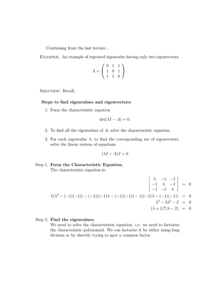
Continuing from the last lecture...
Example. An example of repeated eigenvalue having only two eigenvectors.


0 1 1
A =  1 0 1 .
1 1 0
Solution: Recall,
Steps to find eigenvalues and eigenvectors:
1. Form the characteristic equation
det(λI − A) = 0.
2. To find all the eigenvalues of A, solve the characteristic equation.
3. For each eigenvalue λ, to find the corresponding set of eigenvectors,
solve the linear system of equations
(λI − A)~x = 0
Step 1. Form the Characteristic Equation.
The characteristic equation is:
λ −1 −1 −1 λ −1 = 0
−1 −1 λ λ(λ2 − (−1)(−1)) − (−1)((−1)λ − (−1)(−1)) − 1((−1)λ − (−1)(−1)) = 0
λ3 − 3λ2 − 2 = 0
(λ + 1)2 (λ − 2) = 0
Step 2. Find the eigenvalues.
We need to solve the characteristic equation. i.e. we need to factorize
the characteristic polynomial. We can factorize it by either using long
division or by directly trying to spot a common factor.
Method 1: Long Division.
We want to factorize this cubic polynomial. In general it is quite difficult to guess what the factors may be. We try λ = ±1, ±2, ±3, etc.
and hope to quickly find one factor. Let us try λ = −1. We divide the
polynomial λ3 + 2λ2 − 29λ − 30 by λ + 1, to get,
λ2
3
−λ −2
−3λ −2;
λ + 1 |λ
−λ3 +λ2
−λ2 −3λ
− −λ2 −λ
−2λ
− −2λ
−2
−2
−2
0
The quotient is λ2 − λ − 2.
The remainder is 0.
Therefore λ3 − 3λ − 2 = (λ + 1)(λ2 − λ − 2) + 0.
λ3 − 3λ − 2 = 0
(λ + 1)(λ2 − λ − 2) = 0
(λ + 1)(λ + 1)(λ − 2) = 0
Therefore the eigenvalues are: {−1, 2}.
Method 2: Direct factorization by spotting common factor.
λ −1 −1 −1 λ −1 = 0
−1 −1 λ λ(λ2 − (−1)(−1)) − (−1)((−1)λ − (−1)(−1)) − 1((−1)λ − (−1)(−1))
λ(λ2 − 1) + 1(−λ − 1) − 1(1 + λ)
λ(λ − 1)(λ + 1) − 1(λ + 1) − 1(1 + λ)
(λ + 1)(λ(λ − 1) − 1 − 1)
(λ + 1)(λ2 − λ − 2)
(λ + 1)2 (λ − 2)
Therefore the eigenvalues of A are: {−1, 2}.
=
=
=
=
=
=
0
0
0
0
0
0
Step 3. Find Eigenvectors corresponding to each Eigenvalue:
We now need to find eigenvectors corresponding to each eigenvalue.
case(i) λ1 = −1.
The eigenvectors are the solution space of




x1
−1 −1 −1
 −1 −1 −1   x2  = 
−1 −1 −1
x3
−x1 − x2 − x3 = 0;
the following system:

0
0 
0
x1 = −x2 − x3
The set of eigenvectors corresponding to λ1 = −1 is,


x1
{  x2  |x1 = −x2 − x3 }
x3


−x2 − x3
 | at least one of x2 and x3 is a non-zero real number}
x2
{ 
x3




−1
−1
{ x2  1  + x3  0  | at least one of x2 and x3 is a non-zero real number}
0
1
We therefore can get two linearly independent eigenvectors corresponding
λ1 = −1:
 to 

−1
−1
~v1 =  1 , ~v2 =  0 .
0
1
case(ii) λ2 = 2.
The eigenvectors are the solution space of the following system:



 
2 −1 −1
x1
0
 −1 2 −1   x2  =  0 
−1 −1 2
x3
0
2x1 − x2 − x3 = 0
−x1 + 2x2 − x3 = 0
−x1 − x2 + 2x3 = 0
Since this system of equations looks fairly complicated, it may be
a good idea to use row reduction to simplify the system.




2 −1 −1 0
−1 −1 2 0
↔R1
 −1 2 −1 0  R3→
 −1 2 −1 0 
−1 −1 2 0
2 −1 −1 0


1
1 −2 0
R1 =(−1)R1
 −1 2 −1 0 
→
2 −1 −1 0


1 1 −2 0
R =R2 −2R1
−−3−−−
−−→  0 3 −3 0 
R2 =R1 +R2
0 −3 3 0


1 1 −2 0
R2 =1/3R2
 0 1 −1 0 
→
0 −3 3 0


1 1 −2 0
R3 =R3 +3R2
 0 1 −1 0 
→
0 0 0 0
The resulting set of equations is:
x2 − x3 = 0 =⇒ x2 = x3
x1 + x2 − 2x3 = 0 =⇒ x1 = x3
The set of eigenvectors corresponding to λ2 = 2 is,


x1
{  x2  |x1 = x2 = x3 }
x3


x3
{  x3  |x3 is a non-zero real number}
x3
 
1

1  |x3 is a non-zero real number}
{ x3
1
 
1
An eigenvector corresponding to λ2 = 2 is  1 .
1
Example. An example of a repeated eigenvalue having only one linearly
independent eigenvector.


6 3 −8
A =  0 −2 0  .
1 0 −3
Solution: The characteristic polynomial for A:
λ − 6 −3
8
0
λ+2
0 −1
0
λ+3 (λ − 6)((λ + 2)(λ + 3) − 0) − 3(0 − 0) + 8(0 − (−1)(λ + 2))
λ3 − λ2 − 16λ − 20
(λ + 2)(λ2 − 3λ − 10)
(λ + 2)2 (λ − 5)
= 0
=
=
=
=
Therefore the eigenvalues of A are: λ1 = −2, λ2 = 5.
case(i) λ1 = −2.
The eigenvectors are the solution space of



−8 −3 8
x1
 0
0 0   x2  =
x3
−1 0 1
−x1 + x3 =
−8x1 − 3x2 + 8x3 =
The set of eigenvectors

x1
{  x2
x3

x3

0
{
x3

the following system:
 
0
 0 
0
0 =⇒ x1 = x3
0 =⇒ x2 = 0
corresponding to λ1 = −2 is,

 |x1 = x3 , x2 = 0}

 |x3 is a non-zero real number}

1
{ x3  0  |x3 is a non-zero real number}
1
0
0
0
0

1
An eigenvector corresponding to λ1 = −2 is  0 .
1

case(ii) λ2 = 5.
The eigenvectors are the solution space of



x1
−1 −3 8
 0
7 0   x2  =
−1 0 8
x3
−x1 + 8x3 =
7x2 =
the following system:
 
0
 0 
0
0 =⇒ x1 = 8x3
0 =⇒ x2 = 0
The set of eigenvectors corresponding to λ2 = 5 is,


x1
{  x2  |x1 = 8x3 , x2 = 0}
x3


8x3
{  0  |x3 is a non-zero real number}
x3
 
8

0  |x3 is a non-zero real number}
{ x3
1


8
An eigenvector corresponding to λ2 = 5 is  0 .
1
Example. An example of an eigenvalue repeated three times having only
two linearly independent eigenvectors.


4 0 −1
A =  0 3 0 .
1 0 2
Solution: The characteristic equation for A:
det (λI − A) = 0
λ−4
0
1 0
λ−3
0 = 0
−1
0
λ−2 λ3 − 9λ2 + 27λ − 27 = 0
(λ − 3)3 = 0
Therefore A has only one eigenvalue: λ = 3.
The eigenvectors corresponding to λ = 3 are the solution space of the
following system:

 


0
−1 0 1
x1
 0 0 0   x2  =  0 
x3
0
−1 0 1
−x1 + x3 = 0 =⇒ x1 = x3
The set of eigenvectors corresponding to λ = 3 is,


x1
{  x2  |x1 = x3 }
x3


x3
{  x2  | at least one of x2 and x3 is a non-zero real number}
x3
 
 
0
1
{ x2  1  + x3  0  | at least one on x2 and x3 is a non-zero real number}
0
1
Therefore we can find two linearly independent eigenvectors corresponding
to the eigenvalue λ = 3:
 
 
1
0
 1  and  0  .
1
0
8.3
Dimension of Eigenspace
Definition. The rank of a matrix is defined to be the number of linearly
independent rows or columns.
Remark. We use the following results to determine the rank of a matrix.
• Let A be a square matrix and let Aechelon be the row echelon form of
the matrix. Then both A and Aechelon have the same number of linearly
independent rows.
• Consequently, Rank(A) = Rank(Aechelon ).
• The number of linearly independent rows of a matrix in row echelon
form is just the number of non-zero rows.
• We may conclude that
Rank(A) = Rank(Aechelon ) = number of non-zero rows in Aechelon .

Example.

2. Rank 

3. Rank 



−1 −1 −1
1 1 1
1. Rank  −1 −1 −1  = Rank  0 0 0  = 1.
−1 −1 −1
0 0 0



−8 −3 8
1 0 −1
0
0 0  = Rank  0 −3 0  = 2.
−1 0 1
0 0
0



−1 0 1
−1 0 1
0 0 0  = Rank  0 0 0  = 1.
−1 0 1
0 0 0
Definition. Let A be a square matrix of size n × n having an eigenvalue λ.
The set of eigenvectors corresponding to the eigenvalue λ, alongwith the zero
vector, is called the eigenspace corresponding to eigenvalue λ.
The dimension of the eigenspace is defined to be the maximum number of
linearly independent vectors in the eigenspace.
Theorem Let A be a matrix of size n × n and let λ be an eigenvalue of A
repeating k times. Then the dimension of the eigenspace of λ or equivalently
the maximum number of linearly independent eigenvectors corresponding to
λ is:
n − Rank(λI − A).
Example. Let us use
examples.

0 1
1. Recall A =  1 0
1 1
this result to confirm our calculations in the previous

1
1 
0
• has eigenvalue λ = −1 occurring with multiplicity 2.
• We found two linearly independent eigenvectors corresponding to this
eigenvalue.




−1
−1
~v1 =  1 , ~v2 =  0 .
0
1
We will use the above theorem to confirm that we should indeed expect
to find two linearly independent eigenvectors. By the above theorem, the
maximum number of linearly independent eigenvectors corresponding to
λ = −1 is:
= 3 − Rank(λI − A)


−1 −1 −1
= 3 − Rank  −1 −1 −1 
−1 −1 −1
=3−1
=2


6
3 −8
2. Recall A =  0 −2 0 
−1 0
1
• has eigenvalue λ = −2 occurring with multiplicity 2.
• We found only one linearly independent eigenvector corresponding
to this

 eigenvalue.
1
~v1 =  0 .
1
We will use the above theorem to confirm that we should indeed expect
to find only one linearly independent eigenvector. By the above theorem,
the maximum number of linearly independent eigenvectors corresponding
to λ = −2 is:
= 3 − Rank(λI − A)


−8 −3 8
0 0 
= 3 − Rank  0
−1 0 1
=3−2
=1


4 0 −1
3. Recall A =  0 3 0 
1 0 2
• has eigenvalue λ = 3 occurring with multiplicity 3.
• We found only two linearly independent eigenvectors corresponding
to this
 eigenvalue.

 
0
1



1 , ~v2 =
0 .
~v1 =
0
1
We will use the above theorem to confirm that we should indeed expect to
find only two linearly independent eigenvectors. By the above theorem,
the maximum number of linearly independent eigenvectors corresponding
to λ = 3 is:
= 3 − Rank(λI − A)


−1 0 1
= 3 − Rank  0 0 0 
−1 0 1
=3−1
=2
8.4
Diagonalization
Definition. A square matrix of
the form

d1 0
 0 d2

 . .

 . .

 0 .
0 .
size n is called a diagonal matrix if it is of
. .
0 .
.
.
.
dn−1
. .
0
0
0
.
.
0
dn








Definition. Two square matrices A and B of size n are said to be similar,
if there exists an invertible matrix P such that
B = P −1 AP
Definition. A matrix A is diagonalizable if A is similar to a diagonal matrix. i.e. there exists an invertible matrix P such that P −1 AP = D where D
is a diagonal matrix. In this case, P is called a diagonalizing matrix.
Example. Recall the example we did in the last chapter.
4 2
A=
.
1 3
Solution: In previous lectures we have found,
the eigenvalues of A are: λ1 = 2, λ2 = 5. −1
An eigenvector corresponding to λ1 = 2 is
.
1
2
An eigenvector corresponding to λ2 = 5 is
.
1
Define a new matrix P such that its columns are the eigenvectors of A.
−1 2
P =
.
1 1
Note that since eigenvectors corresponding to distinct eigenvalues are linearly
independent, the columns of P are linearly independent, hence P is an invertible matrix. (We can also confirm this by verifying that the determinant
of P is non-zero).
−1
1 −2
−1
P =
−1 −1
3
P
−1
AP =
=
=
=
−1
1
−1
3
−1
2
−5
3
−1 −6
0
3
2 0
,
0 5
−2
−1
4 2
1 3
−4
−5
−1 2
1 1
0
−15
−1 2
1 1
which is a diagonal matrix. Therefore A is diagonalizable and a diagonalizing
matrix for A is
−1 2
P =
,
1 1
and the corresponding diagonal matrix D is
2 0
D=
.
0 5
Theorem Let A be a square matrix of size n × n. Then A is diagonalizable
if and only if there exists n linearly independent eigenvectors. In this case a
diagonalizing matrix P is formed by taking as its columns the eigenvectors of
A,
P −1 AP = D.
where D is a diagonal matrix whose diagonal entries are eigenvalues corresponding to the eigenvectors of A. The ith diagonal entry is the eigenvalue
corresponding to the eigenvector in the ith column of P .
Example. An example where the matrix

6
3

0 −2
A=
−1 0
is not diagonalizable. Recall

−8
0 .
1
(i) Find the eigenvalues and eigenvectors of A.
(ii) Is A diagonalizable?
(iii) If it is diagonalizable, find a diagonalizing matrix P such that P −1 AP =
D, where D is a diagonal matrix.
Solution: In previous lectures we have found,
A had two eigenvalues:
λ1 = −1 occurring with multiplicity 2, and
λ2 = 5 occurring with multiplicity 1.
We could find only one linearly independent eigenvector corresponding to
λ1 = −1,
and one linearly independent eigenvector corresponding to λ2 = 5.
Therefore we could find only two linearly independent eigenvectors. By the
above theorem, A is not diagonalizable.
Proposition Let A be a square matrix of size n × n. If λ1 and λ2 are two
distinct eigenvalues of A, and ~v1 and ~v2 are eigenvectors corresponding to λ1
and λ2 respectively, then ~v1 and ~v2 are linearly independent.
Corollary Let A be a square matrix of size n. If A has n distinct eigenvalues then A is diagonalizable.
Example. Recall


4
0
1
A =  −1 −6 −2  .
5
0
0
(i) Find the eigenvalues and eigenvectors of A.
(ii) Is A diagonalizable?
(iii) Find a diagonalizing matrix P such that P −1 AP = D, where D is a
diagonal matrix.
Solution: (i) In previous lectures we have found,
The eigenvalues of A are: λ1 = −1, λ2 = −6 
and λ3= 5.
−1
An eigenvector corresponding to λ1 = −1 is 
5
−9
25
1
.

0
An eigenvector corresponding to λ2 = −6 is  1 .
 0
1
.
An eigenvector corresponding to λ3 = 5 is  −3
11
1

(ii) The matrix A is diagonalizable, since A is a square matrix of size 3 × 3
and we have found three linearly independent eigenvectors for A.
(iii) A diagonalizing matrix P has the eigenvectors as its columns. Let
 −1

0
1
5
.
1 −3
P =  −9
25
11
1 0 1
The corresponding diagonal matrix D will have the eigenvalues as diagonal entries corresponding to the columns of P . i.e. the ith diagonal
entry will be the eigenvalue corresponding to the eigenvector in the ith
column.


−1 0 0
D =  0 −6 0  .
0
0 5
We will now verify that P −1 AP = D.

  −1

4
0
1
0
1
5

1 −3
AP =  −1 −6 −2   −9
25
11
5
0
0
1 0 1


1/5 0
5
=  9/25 −6 −15/11 
−1
0
5
 −1


0 1
−1 0 0
5
  0 −6 0 
1 −3
P D =  −9
25
11
1 0 1
0
0 5


1/5 0
5

9/25 −6 −15/11 
=
−1
0
5
AP = P D
(1)
Since the columns of P are linearly independent, P has non-zero determinant and is therefore invertible. We multiply (1) by P −1 on both
sides.
P −1 AP = P −1 P D,
= ID
=D