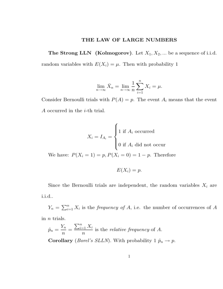
THE LAW OF LARGE NUMBERS
The Strong LLN (Kolmogorov). Let X1 , X2 , ... be a sequence of i.i.d.
random variables with E(Xi ) = µ. Then with probability 1
n
1X
Xi = µ.
lim X̄n = lim
n→∞
n→∞ n
i=1
Consider Bernoulli trials with P (A) = p. The event Ai means that the event
A occurred in the i-th trial.
Xi = IAi =




1 if Ai occurred



0 if Ai did not occur
We have: P (Xi = 1) = p, P (Xi = 0) = 1 − p. Therefore
E(Xi ) = p.
Since the Bernoulli trials are independent, the random variables Xi are
i.i.d..
Yn =
Pn
i=1 Xi
in n trials.
Yn
p̂n =
=
n
is the frequency of A, i.e. the number of occurrences of A
Pn
i=1 Xi
n
is the relative frequency of A.
Corollary (Borel’s SLLN). With probability 1 p̂n → p.
1
The Mean LLN. Let again X1 , X2 , ... be a sequence of i.i.d. random
variables with E(Xi ) = µ. Let Var(Xi ) = σ 2 < ∞.
¸
·
1 Pn
1 Pn
E(X̄n ) = E
X
=
E(Xi ) = µ.
i
n i=1
n i=1
Recall that
We have also
Proposition A. 1. µX̄n = E(X̄n ) = µ.
2
2. σX̄
= V ar(X̄n ) =
n
σ2
n.
·
¸
1 Pn
1 Pn
Proof. 1. E(X̄n ) = E
E(Xi ) = µ.
i=1 Xi =
n
n i=1
£ 1 Pn
¤
σ2
1
2
2
2. σX̄
=
V
ar(
X̄
)
=
V
ar
X
nσ
=
=
2
n
i
i=1
n
n
n
n
£
¤2
The Mean LLN. limn→∞ E X̄n − µ = 0.
£
¤2
V ar(X̄n ) = E X̄n − µ = E
£
¤2
Proof. E X̄n − µ =Var(X̄n ) =
"
n
1X
n
σ2
n
#2
Xi − µ
→ 0 as n → ∞.
i=1
→ 0 as n → ∞.
For Bernoulli trials we have the following statement.
Corollary limn→∞ E[p̂n − p]2 = limn→∞ Var(p̂n ) = 0.
The Weak LLN. (Chebyshev)
limn→∞ X̄n = µ in probability, that is for each ε > 0
2
lim P {|X̄n − µ| > ε} = 0
n→∞
Proof. By the Chebyshev Inequality and the Mean LLN
P {|X̄n − µ| > ε} ≤
V ar(X̄n )
→ 0 as n → 0.
ε2
The case of Bernoulli Trials (Bernoulli): p̂n → p in probability.
3
THE CENTRAL LIMIT THEOREM
Let X1 , X2 , . . . be be a sequence of independent identically distributed
(i.i.d.) random variables.
E(Xi ) = µ, Var(Xi ) = σ 2 < ∞
E
à n
X
!
Xi
=
i=1
n
X
E(Xi ) = nµ,
i=1
Since X1 , X2 , ... are independent
à n
!
n
X
X
Var(Xi ) = nσ 2
Var
Xi =
i=1
i=1
√
σPni=1 Xi = σ n.
Consider the arithmetic mean X̄n =
1
n
Pn
i=1 Xi .
By Proposition A,
µX̄n = µ;
2
σX̄
= V ar(X̄n ) =
n
σ
σX̄n = √ .
n
The random variable
4
σ2
;
n
Pn
Zn =
i=1 Xi − nµ
√
=
σ n
1
n
Pn
i=1 Xi
√σ
n
−µ
=
X̄n − µ
√σ
n
has E(Zn ) = 0, Var(Zn ) = 1.
CLT: FZn (x) → Φ(x) as n → ∞ for any x ∈ (−∞, ∞).
2
This means that the distribution of X̄n is approximately N (µ, σn ) if n is
”large”.
Next page please!
5
Consider Bernoulli Trials with respect to an event A with P (A) = p. Ai
means that A occurred in trial #i. Denote
Xi = IAi =




1 if Ai occurred



0 if Ai did not occur
The number of occurrences in n trials (the frequency of the event A) is
Yn =
n
X
Xi =
i=1
n
X
I AI
i=1
Yn ∼ b(n, p)
E(Xi ) = p, Var(Xi ) = pq, q = 1 − p
E(Yn ) = np, Var(Yn ) = npq, σYn =
The relative frequency of the event A, p̂n =
Yn
n.
r
E(p̂n ) = p, σp̂n =
Pn
Thus Zn =
− nµ Yn − np p̂n − p
= p pq .
= √
npq
σ n
n
√
Corollary. (De Moivre–Laplace).
n→∞
FZn (x) → Φ(x)
6
npq.
Note that
pq
.
n
i=1 Xi
√
for x ∈ (−∞, ∞).
This means that the distribution of p̂n is approximately N (p, pq
n ) if n is
”large”.
7