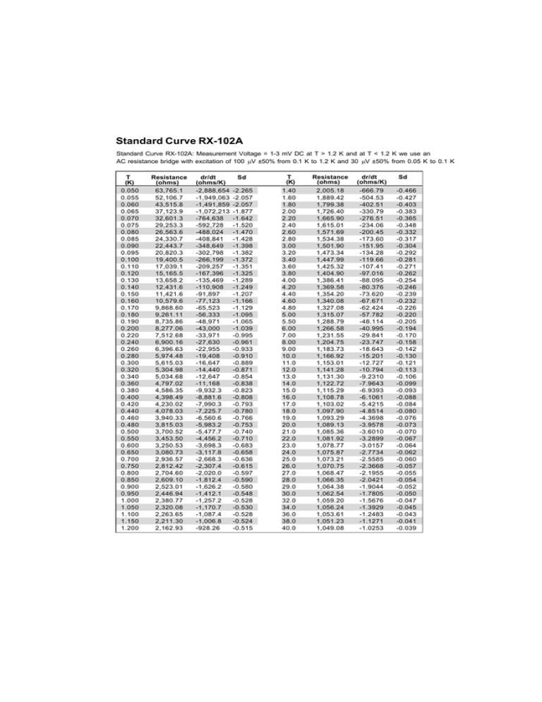
Standard Curve RX-102A
Standard Curve RX-102A: Measurement Voltage = 1-3 mV DC at T > 1.2 K and at T < 1.2 K we use an
AC resistance bridge with excitation of 100 µV ±50% from 0.1 K to 1.2 K and 30 µV ±50% from 0.05 K to 0.1 K
T
(K)
0.050
0.055
0.060
0.065
0.070
0.075
0.080
0.085
0.090
0.095
0.100
0.110
0.120
0.130
0.140
0.150
0.160
0.170
0.180
0.190
0.200
0.220
0.240
0.260
0.280
0.300
0.320
0.340
0.360
0.380
0.400
0.420
0.440
0.460
0.480
0.500
0.550
0.600
0.650
0.700
0.750
0.800
0.850
0.900
0.950
1.000
1.050
1.100
1.150
1.200
Resistance
(ohms)
63,765.1
52,106.7
43,515.8
37,123.9
32,601.3
29,253.3
26,563.6
24,330.7
22,443.7
20,820.3
19,400.5
17,039.1
15,165.5
13,658.2
12,431.6
11,421.6
10,579.6
9,868.60
9,261.11
8,735.86
8,277.06
7,512.68
6,900.16
6,396.63
5,974.48
5,615.03
5,304.98
5,034.68
4,797.02
4,586.35
4,398.49
4,230.02
4,078.03
3,940.33
3,815.03
3,700.52
3,453.50
3,250.53
3,080.73
2,936.57
2,812.42
2,704.60
2,609.10
2,523.01
2,446.94
2,380.77
2,320.08
2,263.65
2,211.30
2,162.93
dr/dt
(ohms/K)
-2,888,654
-1,949,063
-1,491,859
-1,072,213
-764,638
-592,728
-488,024
-408,841
-348,649
-302,798
-266,199
-209,257
-167,396
-135,469
-110,908
-91,897
-77,123
-65,523
-56,333
-48,971
-43,000
-33,971
-27,630
-22,955
-19,408
-16,647
-14,440
-12,647
-11,168
-9,932.3
-8,881.6
-7,990.3
-7,225.7
-6,560.6
-5,983.2
-5,477.7
-4,456.2
-3,698.3
-3,117.8
-2,668.3
-2,307.4
-2,020.0
-1,812.4
-1,626.2
-1,412.1
-1,257.2
-1,170.7
-1,087.4
-1,006.8
-928.26
Sd
T
(K)
Resistance
(ohms)
dr/dt
(ohms/K)
-2.265
-2.057
-2.057
-1.877
-1.642
-1.520
-1.470
-1.428
-1.398
-1.382
-1.372
-1.351
-1.325
-1.289
-1.249
-1.207
-1.166
-1.129
-1.095
-1.065
-1.039
-0.995
-0.961
-0.933
-0.910
-0.889
-0.871
-0.854
-0.838
-0.823
-0.808
-0.793
-0.780
-0.766
-0.753
-0.740
-0.710
-0.683
-0.658
-0.636
-0.615
-0.597
-0.590
-0.580
-0.548
-0.528
-0.530
-0.528
-0.524
-0.515
1.40
1.60
1.80
2.00
2.20
2.40
2.60
2.80
3.00
3.20
3.40
3.60
3.80
4.00
4.20
4.40
4.60
4.80
5.00
5.50
6.00
7.00
8.00
9.00
10.0
11.0
12.0
13.0
14.0
15.0
16.0
17.0
18.0
19.0
20.0
21.0
22.0
23.0
24.0
25.0
26.0
27.0
28.0
29.0
30.0
32.0
34.0
36.0
38.0
40.0
2,005.18
1,889.42
1,799.38
1,726.40
1,665.90
1,615.01
1,571.69
1,534.38
1,501.90
1,473.34
1,447.99
1,425.32
1,404.90
1,386.41
1,369.58
1,354.20
1,340.08
1,327.08
1,315.07
1,288.79
1,266.58
1,231.55
1,204.75
1,183.73
1,166.92
1,153.01
1,141.28
1,131.30
1,122.72
1,115.29
1,108.78
1,103.02
1,097.90
1,093.29
1,089.13
1,085.36
1,081.92
1,078.77
1,075.87
1,073.21
1,070.75
1,068.47
1,066.35
1,064.38
1,062.54
1,059.20
1,056.24
1,053.61
1,051.23
1,049.08
-666.79
-504.53
-402.51
-330.79
-276.51
-234.06
-200.45
-173.60
-151.95
-134.28
-119.66
-107.41
-97.016
-88.095
-80.376
-73.620
-67.671
-62.424
-57.782
-48.114
-40.995
-29.841
-23.747
-18.643
-15.201
-12.727
-10.794
-9.2310
-7.9643
-6.9393
-6.1061
-5.4215
-4.8514
-4.3698
-3.9578
-3.6010
-3.2899
-3.0157
-2.7734
-2.5585
-2.3668
-2.1955
-2.0421
-1.9044
-1.7805
-1.5676
-1.3929
-1.2483
-1.1271
-1.0253
Sd
-0.466
-0.427
-0.403
-0.383
-0.365
-0.348
-0.332
-0.317
-0.304
-0.292
-0.281
-0.271
-0.262
-0.254
-0.246
-0.239
-0.232
-0.226
-0.220
-0.205
-0.194
-0.170
-0.158
-0.142
-0.130
-0.121
-0.113
-0.106
-0.099
-0.093
-0.088
-0.084
-0.080
-0.076
-0.073
-0.070
-0.067
-0.064
-0.062
-0.060
-0.057
-0.055
-0.054
-0.052
-0.050
-0.047
-0.045
-0.043
-0.041
-0.039
Polynomial Representation
Table 1. Chebychev fit coefficients.
Curve RX-102A can be represented by a polynomial equation based on the
Chebycheb polynomials w hich are described below. Three separate
ranges are required to accurately describe the curve, with the parameters
for these ranges given in Table 1. The polynomials represent Curve RX102A on the preceding page with RMS deviations on the order of ±0.5 mK
below 1 K, ±2 mK below 6 K, ±7 mK below 20 K, and ±35 mK below 40 K.
Fit Range: 0.050 K to 0.950 K
Order = 8
A(0)= 0.300923
ZL=3.35453159798
A(1)=-0.401714
ZU=5.00000000000
A(2)= 0.220055
A(3)=-0.098891
A(4)= 0.046804
A(5)=-0.017379
A(6)= 0.009090
A(7)=-0.002703
A(8)= 0.002170
The Chebycheb equation is of the form:
T(x) =
n
∑ a it i (x)
(1)
i= 0
Where T(x) represents the temperature in kelvin, ti(x) is a Chebycheb
polynomial, and a i represents the Chebycheb coefficients. The parameter x
is a normalized variable given by:
(Z − ZL) − (ZU − Z)
x=
(ZU − ZL)
(2)
where Z is the log (base 10) of the resistance and ZL and ZU designate the
log of the lower and upper limit of the resistance over the fit range.
The Chebychev polynomials can be generated from the recursion relation:
t i+ 1 (x) = 2xt i (x) − t i− 1 (x)
(3)
t 0 = 1 , t1 (x) = x
Alternatively, these polynomials are given by:
t1 (x) = cos[ i × arccos( x) ]
(4)
The use of Chebycheb polynomials is no more complicated than the use of
the regular power series and the offer significant advantages in the actual
fitting process. The first step is to transform the measured voltage into the
normalized variable using equation 2. Equation 1 is then used in
combination with Equations 3 and 4 to calculate the temperature. Programs
1 and 2 provide sample BASIC subroutines which will take the resistance
and return the temperature T calculated from Chebychev fits. The
subroutines assume the values ZL and ZU have been input along with the
degree of the fit. The Chebycheb coefficients are also assumed to be in an
array A(0), A(1), …, A(Ndegree).
An interesting property of the Chebychev fit is evident in the form of the
Chebycheb polynomial given in Equation 4. No term in Equation 1 will be
greater than the absolute value of the coefficient. This property makes it
easy to determine the contribution of each term to the temperature
calculation and where to truncate the series if the full accuracy is not
required.
Program 2. BASIC subroutine for evaluating the the temperature T from the
Chebychev series using Equations 1 and 3. An array Tc(Ndegree) must be
defined.
REM Evaluation of Chebychev series
x=((Z-ZL)-ZU-Z))/(ZU-ZL)
Tc(0)=1
Tc(1)=X
T=A(0)+A(1)*X
FOR I=2 to Ndegree
Tc(I)=2*X*Tc(I-1)-Tc(I-2)
T=T+A(I)*Tc(I)
NEXT I
RETURN
Fit Range: 0.950 K to 6.5 K
Order = 9
A(0)= 2.813252
ZL=3.08086045368
A(1)=-2.976371
ZU=3.44910010859
A(2)= 1.299095
A(3)=-0.538334
A(4)= 0.220456
A(5)=-0.090969
A(6)= 0.037095
A(7)=-0.015446
A(8)= 0.005104
A(9)=-0.004254
Fit Range: 6.5 K to 40 K
Order = 9
A(0)= 3074.395992 ZL=2.95500000000
A(1)=-5680.735415 ZU=3.10855552727
A(2)= 4510.873058
A(3)=-3070.206226
A(4)= 1775.293345
A(5)= -857.606658
A(6)= 336.220971
A(7)= -101.617491
A(8)=
21.390256
A(9)=
-2.407847
Program 2. BASIC subroutine for evaluating the
temperature T from the Chebychev series using
Equations 1 and 4.
REM Evaluation of Chebychev series
x=((Z-ZL)-ZU-Z))/(ZU-ZL)
T=0
FOR I=0 to Ndegree
T=T+A(I)*COS(I*ARCCOS(X))
NEXT I
RETURN