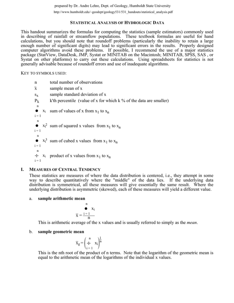
prepared by Dr. Andre Lehre, Dept. of Geology, Humboldt State University
http://www.humboldt.edu/~geodept/geology531/531_handouts/statistical_analysis.pdf
STATISTICAL ANALYSIS OF HYDROLOGIC DATA
This handout summarizes the formulas for computing the statistics (sample estimators) commonly used
in describing of rainfall or streamflow populations. These textbook formulas are useful for hand
calculations, but you should note that roundoff problems (particularly the inability to retain a large
enough number of significant digits) may lead to significant errors in the results. Properly designed
computer algorithms avoid these problems. If possible, I recommend the use of a major statistics
package (StatView, DataDesk, JMP, Systat or MINITAB on the Macintosh; MINITAB, SPSS, SAS , or
Systat on other platforms) to carry out these calculations. Using spreadsheets for statistics is not
generally advisable because of roundoff errors and use of inadequate algorithms.
KEY TO SYMBOLS USED:
n
x
sx
Pk
total number of observations
sample mean of x
sample standard deviation of x
k'th percentile (value of x for which k % of the data are smaller)
n
∑
xi sum of values of x from x1 to xn
∑
xi2 sum of squared x values from x1 to xn
∑
xi3 sum of cubed x values from x1 to xn
∏
xi product of x values from x1 to xn
i=1
n
i=1
n
i=1
n
i=1
I.
MEASURES OF CENTRAL TENDENCY
These statistics are measures of where the data distribution is centered, i.e., they attempt in some
way to describe quantitatively where the "middle" of the data lies. If the underlying data
distribution is symmetrical, all these measures will give essentially the same result. Where the
underlying distribution is asymmetric (skewed), each of these measures will yield a different value.
a.
sample arithmetic mean
n
∑
x=
xi
i=1
n
This is arithmetic average of the x values and is usually referred to simply as the mean.
b.
sample geometric mean
n
xg =
∏
xi
1
n
i=1
This is the nth root of the product of n terms. Note that the logarithm of the geometric mean is
equal to the arithmetic mean of the logarithms of the individual x values.
c.
sample harmonic mean
xh =
n
n
∑
i=1
1
xi
This is the reciprocal of the mean value of the reciprocals of individual values.
d.
sample median
xmd = 50th percentile of data
This is the middle value of a data series: half of the values are larger than this number, and half
are smaller. If the data series consists of an even number of values, the median is the average
of the two middle values.
e.
sample mode
xmo = most frequent value
This is the value which occurs most frequently in a data series. If there is no most frequent
value, the data series is modeless. If there are two or more most frequent values, the
distribution is bimodal or multimodal.
The arithmetic mean is the most commonly used measure of central tendency on account of its
computational simplicity and general sampling stability. The US Weather Bureau uses the mean as
as the precipitation normal. However, in significantly skewed distributions the mean may be
misleading and the median is a better indicator of the center of the distribution.
II. MEASURES OF VARIABILITY OR DISPERSION
a.
sample standard deviation
n
n
∑
sx =
∑
n
∑
xi - x 2
i=1
n-1
=
xi2 -
2
xi
i=1
i=1
n
n-1
The sample standard deviation is the square root of the mean squared difference between each
observation and the sample mean; it is defined by the left-most formula above. This formula is
awkward for hand computations, but minimizes roundoff errors. The equation is usually
reorganized into the form on the right for hand calculations.
b.
sample variance
sx2 = square of the sample standard deviation
c.
graphical standard deviation
Sgr = P 84 - P16
2
The graphical standard deviation is a quick approximation of the sample standard deviation
based on the cumulative curve. P 84 and P16 are the 84th and 16th percentiles of the data as
read from the cumulative frequency curve plotted on probability paper.
9
8
7
P84
6
5
4
P16
3
2
.01
.1
1
5 10 20 30
50
70 80 90 95
99
99.9 99.99
% ≤ indicated value
d.
sample range
sample range = xmax -xmin
The sample range is the difference between the maximum and minimum values in a data set.
e.
sample coefficient of variation
Cv = s x
x
The sample coefficient of variation is the ratio of the sample standard deviation to the sample
mean. It is useful in comparing data sets where the variability of the data increases markedly
with an increase in the mean.
III. MEASURES OF ASYMMETRY OR SKEWNESS
a.
sample skewness
n
a=
n
n-1 n-2
n
∑
xi -x 3 =
i=1
n2
n-1 n-2
∑
i=1
n
n
∑
xi3
-3
i=1
n
xi2
x + 2x3
The sample skewness measures the degree to which a distribution is asymmetric. Symmetric
distributions have zero skewness. Distributions with a tail to the right yield positive (+) values
of skew, while those with a left tail yield negative (–) values. Values of raw skewness are
often very large and hard to interpret; the sample coefficient of skewness, below, is more
commonly used.
b.
sample coefficient of skewness
Cs = a
sx3
The sample coefficient of skewness is the ratio of the sample skewness to the cube of the
sample standard deviation. For symmetrical distributions C s = 0. If Cs > 0, the distribution is
asymmetric with a tail extending to the right (right skew); if Cs < 0, the distribution is
asymmetric with a tail extending to the left (left skew). The larger the absolute value of Cs, the
more asymmetric the distribution.
c.
Pearson's sample skewness
Sk = x -sxmo
x
This is another commonly used measure of skewness. It is much easier to calculate by hand
than the ordinary sample skewness.
mean
median
mode
symmetrical distribution: skew = 0
mode
median
mean
asymmetric distribution: positive (right) skew
IV. CONFIDENCE LIMITS
a.
(1- ) x 100% confidence limits on the mean
s
CI = x ± t n−1,α /2 x
n
t n−1,α /2 is the value of the t-statistic from tables, where n-1 is the degrees of freedom and
(α/2) is typically 0.025 (i.e, α = 0.05). If n is "large enough" (typically n ≥ 25 -30) we can
substitute zα/2 in place of the t - value.
Confidence limits on the mean allow us to assess the degree of uncertainty likely in our using
the sample mean x to estimate the population mean µ. For example, if we construct a (1-α) =
95% confidence interval around the sample mean, we can have 95% confidence that the true
population mean lies in that interval. That is, 95 times out of 100 an interval constructed from
our sample in this fashion will contain the true population mean.