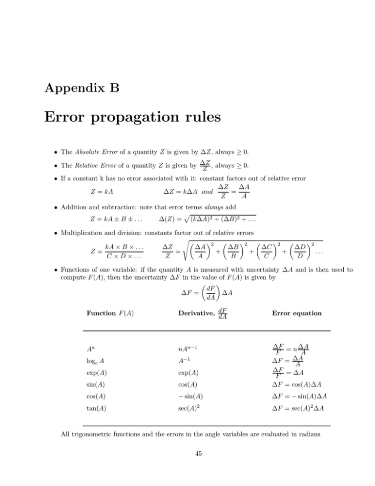
Appendix B
Error propagation rules
• The Absolute Error of a quantity Z is given by ∆Z, always ≥ 0.
• The Relative Error of a quantity Z is given by ∆Z
Z , always ≥ 0.
• If a constant k has no error associated with it: constant factors out of relative error
∆A
∆Z
=
Z = kA
∆Z = k∆A and
Z
A
• Addition and subtraction: note that error terms always add
p
Z = kA ± B ± . . .
∆(Z) = (k∆A)2 + (∆B)2 + . . .
• Multiplication and division: constants factor out of relative errors
s
∆B 2
∆C 2
∆D 2
∆Z
∆A 2
kA × B × . . .
+
+
+
...
=
Z=
C × D × ...
Z
A
B
C
D
• Functions of one variable: if the quantity A is measured with uncertainty ∆A and is then used to
compute F (A), then the uncertainty ∆F in the value of F (A) is given by
dF
∆F =
∆A
dA
Function F (A)
Derivative, dF
dA
Error equation
An
nAn−1
loge A
A−1
exp(A)
exp(A)
sin(A)
cos(A)
∆F
F
∆F
∆F
F
∆F
cos(A)
− sin(A)
∆F = − sin(A)∆A
tan(A)
sec(A)2
∆F = sec(A)2 ∆A
= n ∆A
A
= ∆A
A
= ∆A
= cos(A)∆A
All trigonometric functions and the errors in the angle variables are evaluated in radians
45
46
APPENDIX B. ERROR PROPAGATION RULES
How to derive an error equation
Let’s use the change of variable method to determine the error equation for the following expression:
Mp
0.5 kx (1 − sin θ)
m
y=
(B.1)
• Begin by rewriting Equation B.1 as a product of terms:
y = M ∗ m−1 ∗ [ 0.5 ∗ k ∗ x ∗ (1 − sin θ)]
= M ∗ m
−1
1/2
∗ 0.5
∗ k
1/2
∗ x
1/2
1/2
(B.2)
1/2
∗ (1 − sin θ)
(B.3)
• Assign to each term in Equation B.3 a new variable name A, B, C, . . . , then express v in terms of
these new variables,
y=A ∗ B ∗ C ∗ D ∗ E ∗ F
(B.4)
• With ∆(y) representing the error or uncertainty in the magnitude of y, the error expression for y is
easily obtained by applying Rule 4 to the product of terms Equation B.4:
∆(y)
=
y
s
∆(A)
A
2
+
∆(B)
B
2
+
∆(C)
C
2
+
∆(D)
D
2
+
∆(E)
E
2
+
∆(F )
F
2
(B.5)
• Select from the table of error rules an appropriate error expression for each of these new variables as
shown below. Note that F requires further simplification since there are two terms under the square
root, so we equate these to a variable G:
A = M,
∆(A) = ∆(M )
B = m−1 ,
∆(m)
∆(B)
∆(m)
B = −1 m = − m
C = 0.51/2 ,
∆(C)
C =
1
2
D = k1/2 ,
∆(D)
D =
1
2
∆(0.5)
=0
|0.5|
∆(k)
∆(k)
=
k
2k
E = x1/2 ,
∆(E)
E =
1
2
∆(x)
∆(x)
x = 2x
F = G1/2 ,
∆(F )
F =
1
2
∆(G)
∆(G)
G = 2G
G = 1 − sin θ,
∆(G) =
p
(∆(1))2 + (∆(sin θ))2 = cos θ∆θ
• Finally, replace the error terms into the original error Equation B.5, simplify and solve for ∆(y) by
multiplying both sides of the equation with y:
∆(y) = y
s
∆M
M
2
+
∆m
m
2
+
∆k
2k
2
+
∆x
2x
2
+
cos θ∆θ
2 − 2 sin θ
2
(B.6)