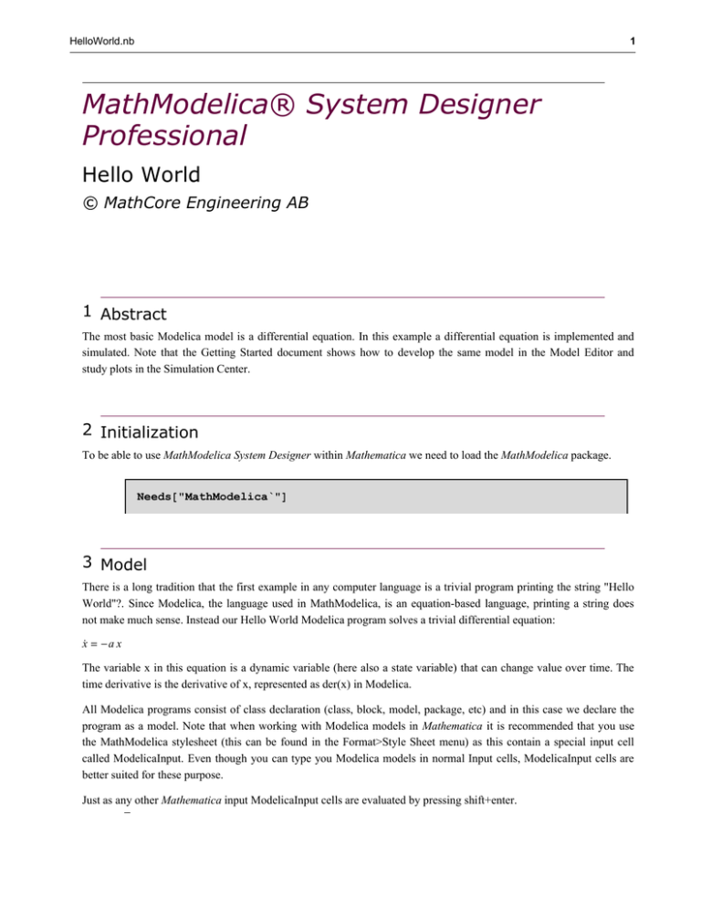
HelloWorld.nb
1
MathModelica® System Designer
Professional
Hello World
© MathCore Engineering AB
1 Abstract
The most basic Modelica model is a differential equation. In this example a differential equation is implemented and
simulated. Note that the Getting Started document shows how to develop the same model in the Model Editor and
study plots in the Simulation Center.
2 Initialization
To be able to use MathModelica System Designer within Mathematica we need to load the MathModelica package.
Needs@"MathModelica`"D
3 Model
There is a long tradition that the first example in any computer language is a trivial program printing the string "Hello
World"?. Since Modelica, the language used in MathModelica, is an equation-based language, printing a string does
not make much sense. Instead our Hello World Modelica program solves a trivial differential equation:
x° = -a x
The variable x in this equation is a dynamic variable (here also a state variable) that can change value over time. The
time derivative is the derivative of x, represented as der(x) in Modelica.
All Modelica programs consist of class declaration (class, block, model, package, etc) and in this case we declare the
program as a model. Note that when working with Modelica models in Mathematica it is recommended that you use
the MathModelica stylesheet (this can be found in the Format>Style Sheet menu) as this contain a special input cell
called ModelicaInput. Even though you can type you Modelica models in normal Input cells, ModelicaInput cells are
better suited for these purpose.
Just as any other Mathematica input ModelicaInput cells are evaluated by pressing shift+enter.
HelloWorld.nb
2
model HelloWorld
Real x(start=1);
equation
der(x)=-x;
end HelloWorld;
4 Simulation
The MathModelica System Designer Professional command Simulate simulates the model given by the Modelica code
given above.
?? Simulate
Simulate@model,8t,tmin,tmax<D
simulates the model in the range tmin to tmax.
Attributes@SimulateD = 8ReadProtected<
Options@SimulateD = 8Method → Dassl, Tolerance → 0.0001,
IntervalLength → 0, NumberOfIntervals → 500, InitialValues → 8<,
ParameterValues → 8<, InteractiveVariables → True<
We simulate the HelloWorld example.
Simulate@HelloWorld, 8t, 0, 10<D
<SimulationData: : : 80., 10.< :
504 data points : 1 events : 2 variables>
8x, x <
The Simulate command returns a SimulationData object containing all model parameters and variables in the form of
interpolating functions. It is possible to use the Mathematica Plot command to plot simulation results.
HelloWorld.nb
3
Plot@x@tD, 8t, 0, 10<D;
0.3
0.2
0.1
2
4
6
8
10
However, it is better to use the PlotSimulation command as this is especially adapted to handle simulation results,
including the possibility to plot simulation results from several different simulations, using the SimulationResult
option, in the same plot, as well as the possibility to plot hierarchical variables, which are very often used in modeling.
? PlotSimulation
PlotSimulation@f,8t,tmin,tmax<D generates a plot
of the signal f as a function of t from tmin to tmax.
PlotSimulation@8f1,f2,...<,8t,tmin,tmax<D plots several
functions fi. PlotSimulation@8"var1","var2"<,8t,tmin,tmax<D
plots variables having the Modelica names var1 and var2.
PlotSimulation@f,8t,tmin,tmax<,SimulationResult−>resD
generates a plot of f using simulation result res. Default
value of res is the result from the latest simulation.
HelloWorld.nb
4
PlotSimulation@x@tD, 8t, 0, 10<D;
x@tD
1
0.8
0.6
0.4
0.2
t
2
4
6
8
10
In many cases you want to compare results for different simulations, for instance you might want to test different initial
or parameter values.
?? Simulate
Simulate@model,8t,tmin,tmax<D
simulates the model in the range tmin to tmax.
Attributes@SimulateD = 8ReadProtected<
Options@SimulateD = 8Method → Dassl, Tolerance → 0.0001,
IntervalLength → 0, NumberOfIntervals → 500, InitialValues → 8<,
ParameterValues → 8<, InteractiveVariables → True<
We can make several simulations and store the results in different variables.
res1 = Simulate@HelloWorld, 8t, 0, 10<D;
res2 = Simulate@HelloWorld, 8t, 0, 10<, InitialValues → 8x
res3 = Simulate@HelloWorld, 8t, 0, 10<, InitialValues → 8x
Then we can use the SimulationResult option to compare the results in one plot.
−10<D;
10<D;
HelloWorld.nb
5
PlotSimulation@x@tD, 8t, 0, 10<, SimulationResult → 8res1, res2, res3<D;
x@tD
x@tD
x@tD
10
5
t
2
-5
-10
4
6
8
10