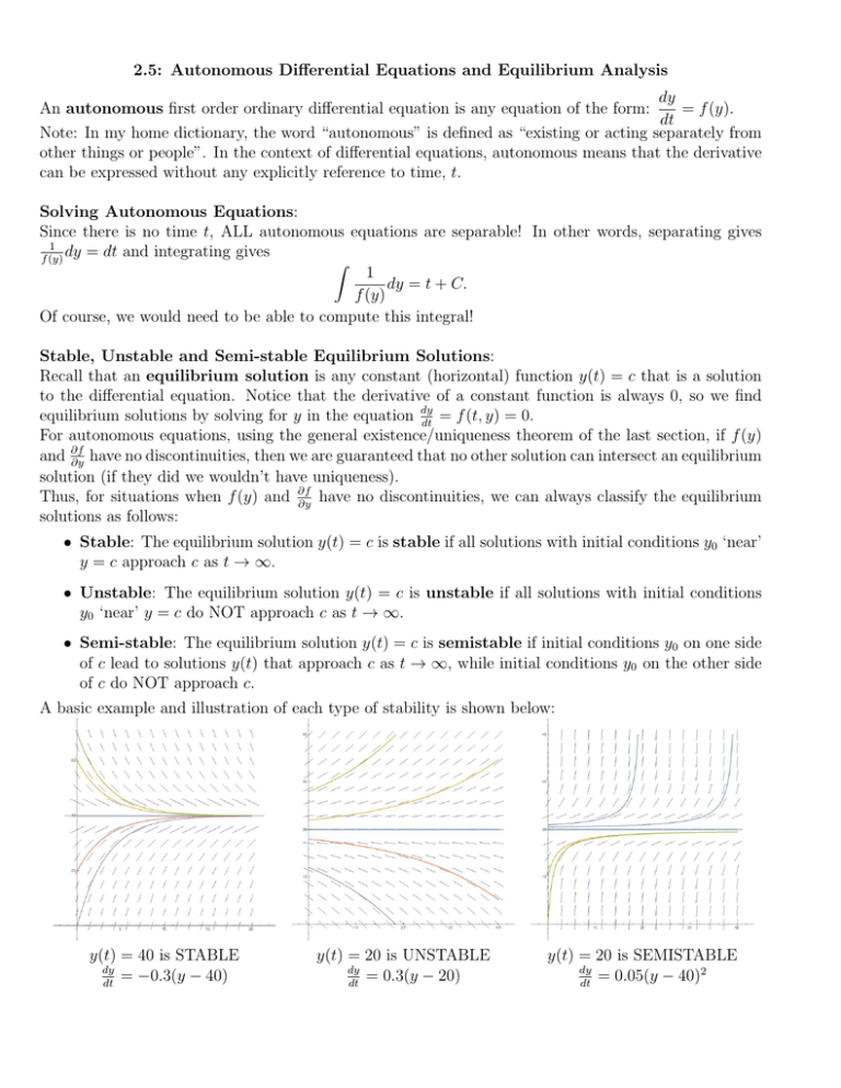
2.5: Autonomous Differential Equations and Equilibrium Analysis
dy
= f (y).
An autonomous first order ordinary differential equation is any equation of the form:
dt
Note: In my home dictionary, the word “autonomous” is defined as “existing or acting separately from
other things or people”. In the context of differential equations, autonomous means that the derivative
can be expressed without any explicitly reference to time, t.
Solving Autonomous Equations:
Since there is no time t, ALL autonomous equations are separable! In other words, separating gives
1
dy = dt and integrating gives
f (y)
Z
1
dy = t + C.
f (y)
Of course, we would need to be able to compute this integral!
Stable, Unstable and Semi-stable Equilibrium Solutions:
Recall that an equilibrium solution is any constant (horizontal) function y(t) = c that is a solution
to the differential equation. Notice that the derivative of a constant function is always 0, so we find
= f (t, y) = 0.
equilibrium solutions by solving for y in the equation dy
dt
For autonomous equations, using the general existence/uniqueness theorem of the last section, if f (y)
have no discontinuities, then we are guaranteed that no other solution can intersect an equilibrium
and ∂f
∂y
solution (if they did we wouldn’t have uniqueness).
have no discontinuities, we can always classify the equilibrium
Thus, for situations when f (y) and ∂f
∂y
solutions as follows:
• Stable: The equilibrium solution y(t) = c is stable if all solutions with initial conditions y0 ‘near’
y = c approach c as t → ∞.
• Unstable: The equilibrium solution y(t) = c is unstable if all solutions with initial conditions
y0 ‘near’ y = c do NOT approach c as t → ∞.
• Semi-stable: The equilibrium solution y(t) = c is semistable if initial conditions y0 on one side
of c lead to solutions y(t) that approach c as t → ∞, while initial conditions y0 on the other side
of c do NOT approach c.
A basic example and illustration of each type of stability is shown below:
y(t) = 40 is STABLE
dy
= −0.3(y − 40)
dt
y(t) = 20 is UNSTABLE
dy
= 0.3(y − 20)
dt
y(t) = 20 is SEMISTABLE
dy
= 0.05(y − 40)2
dt
Classifying Equilibrium Solutions:
dy
= f (y). (and assuming f and
Given
dt
∂f
∂y
are continuous)
1. Solve f (y) = 0 to get the equilibrium solutions.
2. Study f (y) around the equilibrium values as follows (drawing f (y) might help):
(a) Draw a vertical line (the phase line) and make tick marks at equilibrium values.
(b) Between tick marks determine if f (y) is positive or negative.
(c) If f (y) is positive, then
(d) If f (y) is negative, then
dy
dt
dy
dt
will be positive so any solution in this region will be increasing.
will be negative so any solution in this region will be decreasing.
3. Classify:
(a) Increasing below and decreasing above =⇒ stable.
(b) Decreasing below and increasing above =⇒ unstable.
(c) Decreasing below and above OR increasing below and above =⇒ semistable.
Examples:
1. Find and classify the equilibrium points of
dy
dt
= (1 − y)(3 − y).
(a) y(t) = 1 and y(t) = 3 are the equilibrium solutions.
(b) For y > 3: dy
is positive, so y(t) is increasing.
dt
is negative, so y(t) is decreasing.
For 1 < y < 3: dy
dt
dy
For y < 1: dt is positive, so y(t) is increasing.
(c) Thus, y(t) = 1 is stable. And y(t) = 3 is unstable.
2. Find and classify the equilibrium points of
dy
dt
= −(y − 10)2 (y − 4).
(a) y(t) = 4 and y(t) = 10 are the equilibrium solutions.
(b) For y > 10: dy
is negative, so y(t) is decreasing.
dt
For 4 < y < 10: dy
is negative , so y(t) is decreasing.
dt
dy
For y < 4: dt is positive, so y(t) is increasing.
(c) Thus, y(t) = 4 is stable. And y(t) = 10 is semistable.
3. Find and classify the equilibrium points of
dy
dt
= (y 3 − 8)(ey − 1).
(a) y(t) = 0, y(t) = 2 are the equilibrium solutions.
(b) For y > 2: dy
is positive, so y(t) is increasing.
dt
For 0 < y < 2: dy
is negative, so y(t) is decreasing.
dt
dy
For y < 0: dt is positive, so y(t) is increasing.
(c) Thus, y(t) = 0 is stable. And y(t) = 2 is unstable.
Population Dynamics:
Typically, the rate of change of a population is only dependent on the current population size in some
way. Thus, the differential equation for a population is typically time-independent (so it is autonomous).
The study of populations is a big application of differential equations that we have been waiting to discuss
until now.
1. Let y = y(t) = the size of the population at time t.
This could be any organism (people, people that have disease, people that know a rumor, bugs,
bacteria, fish, other animals, plants, ...).
dy
= rate of change of population with respect to time.
dt
For example, if y is in bacteria and t is in minutes, then the units of dy
will be bacteria/minute.
dt
dy
So dt can, roughly, be thought of as the number of bacteria that will be added to the population
over the next minute (I say ‘roughly’ because it actually is the instantaneous rate which is not
exactly the same as the average rate over the next minute, but they would be very, very close).
2. Thus,
We considered three models in lecture:
• Unrestricted (Natural) Growth:
dy
= ry
dt
– Plenty of food and space. Assumes: “The rate of change of the population proportional to
the population size.”
– r = relative growth rate (decimal version of the percentage growth per time). So ry is the
approximate number of people added to the population each year.
– The solution is exponential.
– There is only one equilibrium at y(t) = 0 and, for positive r, it is unstable.
y
dy
=r 1−
y, with 0 < K and r > 0.
• Logistic Growth:
dt
K
– Initially like unrestricted growth, but there is a carrying capacity K that the population size
can’t exceed.
– For positive r, there are two equilibrium at y(t) = 0 which is unstable and y(t) = K which
is stable.
dy
y y
= −r 1 −
1−
y with 0 < T < K, r > 0
• Logistic Growth with a Threshold:
dt
K
T
– If the population size is below a certain threshold size, T , then the population will decrease
to zero. If the population is above this threshold, then the population behaves like logistic
growth.
– For positive r, there are three equilibrium at y(t) = 0 which is stable, y(t) = T which is
unstable, and y(t) = K which is stable.