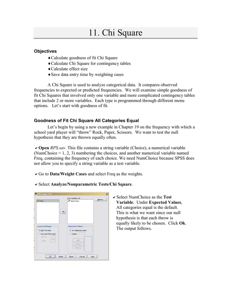
11. Chi Square
Objectives
Calculate goodness of fit Chi Square
Calculate Chi Square for contingency tables
Calculate effect size
Save data entry time by weighting cases
A Chi Square is used to analyze categorical data. It compares observed
frequencies to expected or predicted frequencies. We will examine simple goodness of
fit Chi Squares that involved only one variable and more complicated contingency tables
that include 2 or more variables. Each type is programmed through different menu
options. Let’s start with goodness of fit.
Goodness of Fit Chi Square All Categories Equal
Let’s begin by using a new example in Chapter 19 on the frequency with which a
school yard player will “throw” Rock, Paper, Scissors. We want to test the null
hypothesis that they are thrown equally often.
Open RPS.sav. This file contains a string variable (Choice), a numerical variable
(NumChoice = 1, 2, 3) numbering the choices, and another numerical variable named
Freq, containing the frequency of each choice. We need NumChoice because SPSS does
not allow you to specify a string variable as a test variable.
Go to Data/Weight Cases and select Freq as the weights.
Select Analyze/Nonparametric Tests/Chi Square.
Select NumChoice as the Test
Variable. Under Expected Values,
All categories equal is the default.
This is what we want since our null
hypothesis is that each throw is
equally likely to be chosen. Click Ok.
The output follows.
Chi-Square Test
Frequencies
As you can see, the expected values were 25 each, just as we expected. Now,
compare this Chi Square to the value computed in the text. Once again, they are in
agreement.
Goodness of Fit Chi Square Categories Unequal
Now, let’s try an example where the expected values are not equal across
categories. The difference is we have to specify the expected proportions. This example
is based on Exercise 19.3 in the text, but the numbers in the data set are slightly different.
In the exercise, Howell discusses his theory that when asked to sort one-sentence
characteristics like “I eat too fast” into piles ranging from “not at all like me” to “very
much like me,” the percentage of items placed in each pile will be approximately 10%,
20%, 40%, 20%, and 10%. In our data set, the frequencies are 7, 11, 21 ,7, and 4
respectively.
Open unequal categories.sav. There is no need to save RPS.sav since we did not
change the data file in anyway.
Choose Data/Weight Cases and use Frequency as the weighting variable.
Select Analyze/Nonparametric Statistics/Chi Square.
Select Category as the Test
Variable. Under Expected Values,
select Values. Now, we have to type
in the expected proportion of cases
that should fit each category. Note
that even those it requests
expected values, it really wants
expected proportions. These must
be specified in order to match the
ascending numeric order of the
categories in our data files (e.g., 1 =
not at all like to 5 = very much like).
So, type 10, click Add. Type 20,
click Add, etc. Then, click Ok. The
output follows.
Chi-Square Test
Frequencies
RATING
not at all like me
somewhat unlike me
neither like me or
unlike me
somewhat like me
v ery much like me
Total
Observ ed N
7
11
Expected N
5.0
10.0
Residual
2.0
1.0
21
20.0
1.0
7
4
50
10.0
5.0
-3.0
-1.0
Test Statistics
Chi-Square a
df
Asy mp. Sig.
RATING
2.050
4
.727
a. 0 cells (.0%) hav e expected f requencies less than
5. The minimum expected cell f requency is 5.0.
As you can see, SPSS calculated the expected values based on the proportions that
we indicated-check the math if you would like. In this case, the fact that the Chi Square
is not significant supports the hypothesis. The observed frequencies of ratings fit with
the predicted frequencies.
Chi Square for Contingency Tables
Let’s use an example illustrated in the text. We want to examine the hypothesis
that Prozac is an effect treatment to keep anorexics from relapsing.
As you can see the data are nicely displayed in Table 19.4 in the text.
Select File/New/Data.
In Variable View, create two variables. Name one fault and specify the Values such
that 1 = low fault and 2 = high fault. Name the other variable verdict and specify the
Values such that 1= guilty and 2 = not guilty. Then return to the Data View.
There are four possible combinations of the two variables, as illustrated in the text.
They are Drug/Success, Drug/Relapse, Placebo/Success, and Placebo/Relapse. So,
enter 1,1,2, 2 under Drug and 1, 2, 1, 2 under Outcome, in the first four rows. Then
add a column labeled Freq containing the frequencies for each cell. A sample follows.
Select Data/Weight Cases.
Select Weight cases by and
select counts as the Frequency
Variable. Click Ok. Until we
turn this off, SPSS will run
analyses based on the
frequencies we have specified
here.
Select Analyze/Descriptive Statistics/Crosstabs.
To be consistent with the
presentation in the text, select
Treatment for Rows and
Outcome for Columns. Select
Display clustered bar charts
to help us visualize the data.
Click on Statistics.
Select Chi-square, and then click Continue.
(One would have thought that chi-square
would be the default, but oddly enough it
isn’t. Under Nominal, select Phi and
Cramer’s V as well so we can get a measure
of effect size. In the main dialog box, click
on Cells.
Under Count, select Observed and
Expected. Under Percentages, select Row,
Column, and Total. Then click Continue.
In the main dialog box, click Ok. The output
follows.
Compare the Expected Counts to the values in the text. Finally, compare the Chi Square
values. We are interested in the Pearson Chi Square because it was calculated the same
way as the one in the textbook. Once again, the results are consistent with the textbook.
In this chapter you learned to use SPSS to calculate Goodness of Fit tests with and
without equal frequencies. You also learned to calculate Chi Square for contingency
tables, and learned a trick to reduce data entry by weighting cases. Complete the
following exercises to help you become familiar with these commands.
Exercises
1. Using alley chosen.sav, use a Goodness of Fit Chi Square to test the hypothesis
that rats are more likely than chance to choose Alley D.
2. Solve Exercise 19.3 from the textbook using SPSS. Create the data file yourself.
3. Create your own data file to represent the observed data presented in the textbook
in Table 19.2 using Weight Cases.
4. Using the data file you created in Exercise 3, calculate a Chi Square using
crosstabs to examine the hypothesis that the number of bystanders is related to
seeking assistance. Be sure to calculate Cramer’s Phi. Compare your results to
the textbook.