1
CHAPTER 1
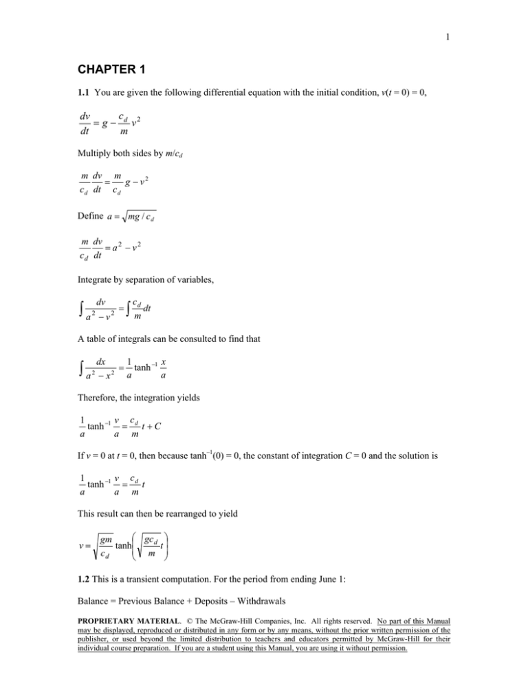
1.1 You are given the following differential equation with the initial condition, v(t = 0) = 0,
c
dv
= g − d v2
dt
m
Multiply both sides by m/cd
m dv m
=
g − v2
c d dt c d
Define a = mg / c d
m dv
= a2 − v2
c d dt
Integrate by separation of variables,
dv
cd
∫ a 2 − v 2 = ∫ m dt
A table of integrals can be consulted to find that
∫a
2
1
dx
x
= tanh −1
2
a
a
−x
Therefore, the integration yields
1
v c
tanh −1 = d t + C
a
a m
If v = 0 at t = 0, then because tanh–1(0) = 0, the constant of integration C = 0 and the solution is
1
v c
tanh −1 = d t
a
a m
This result can then be rearranged to yield
v=
⎛ gc d ⎞
gm
t⎟
tanh⎜
⎜ m ⎟
cd
⎝
⎠
1.2 This is a transient computation. For the period from ending June 1:
Balance = Previous Balance + Deposits – Withdrawals
PROPRIETARY MATERIAL. © The McGraw-Hill Companies, Inc. All rights reserved. No part of this Manual
may be displayed, reproduced or distributed in any form or by any means, without the prior written permission of the
publisher, or used beyond the limited distribution to teachers and educators permitted by McGraw-Hill for their
individual course preparation. If you are a student using this Manual, you are using it without permission.
2
Balance = 1512.33 + 220.13 – 327.26 = 1405.20
The balances for the remainder of the periods can be computed in a similar fashion as tabulated
below:
Date
Deposit
Withdrawal
1-May
Balance
$ 1512.33
$ 220.13
$ 327.26
$ 216.80
$ 378.61
$ 450.25
$ 106.80
$ 127.31
$ 350.61
1-Jun
$ 1405.20
1-Jul
$ 1243.39
1-Aug
$ 1586.84
1-Sep
$ 1363.54
1.3 At t = 12 s, the analytical solution is 50.6175 (Example 1.1). The numerical results are:
step
1
0.5
absolute
relative error
1.15%
0.61%
v(12)
51.2008
50.9259
where the relative error is calculated with
absolute relative error =
analytical − numerical
× 100%
analytical
The error versus step size can be plotted as
2.0%
1.0%
relative error
0.0%
0
0.5
1
1.5
2
2.5
Thus, halving the step size approximately halves the error.
1.4 (a) The force balance is
PROPRIETARY MATERIAL. © The McGraw-Hill Companies, Inc. All rights reserved. No part of this Manual
may be displayed, reproduced or distributed in any form or by any means, without the prior written permission of the
publisher, or used beyond the limited distribution to teachers and educators permitted by McGraw-Hill for their
individual course preparation. If you are a student using this Manual, you are using it without permission.
3
dv
c'
=g− v
dt
m
Applying Laplace transforms,
sV − v(0) =
g c'
− V
s m
Solve for
V=
g
v(0)
+
s ( s + c ' / m) s + c ' / m
(1)
The first term to the right of the equal sign can be evaluated by a partial fraction expansion,
g
A
B
= +
s ( s + c ' / m) s s + c ' / m
(2)
g
A( s + c' / m) + Bs
=
s ( s + c ' / m)
s ( s + c ' / m)
Equating like terms in the numerators yields
A+ B=0
g=
c'
A
m
Therefore,
A=
mg
c'
B=−
mg
c'
These results can be substituted into Eq. (2), and the result can be substituted back into Eq. (1) to
give
V=
mg / c'
mg / c'
v(0)
−
+
s
s + c' / m s + c' / m
Applying inverse Laplace transforms yields
v=
mg mg −( c '/ m )t
−
e
+ v(0)e −( c '/ m )t
c'
c'
or
PROPRIETARY MATERIAL. © The McGraw-Hill Companies, Inc. All rights reserved. No part of this Manual
may be displayed, reproduced or distributed in any form or by any means, without the prior written permission of the
publisher, or used beyond the limited distribution to teachers and educators permitted by McGraw-Hill for their
individual course preparation. If you are a student using this Manual, you are using it without permission.
4
v = v(0)e −( c '/ m )t +
(
mg
1 − e −( c '/ m )t
c'
)
where the first term to the right of the equal sign is the general solution and the second is the
particular solution. For our case, v(0) = 0, so the final solution is
v=
(
mg
1 − e −( c '/ m )t
c'
)
(b) The numerical solution can be implemented as
12.5 ⎤
⎡
v(2) = 0 + ⎢9.81 −
(0) 2 = 19.62
68.1 ⎥⎦
⎣
12.5
⎡
⎤
v(4) = 19.62 + ⎢9.81 −
(19.62)⎥ 2 = 32.0374
68.1
⎣
⎦
The computation can be continued and the results summarized and plotted as:
t
0
2
4
6
8
10
12
v
0
19.6200
32.0374
39.8962
44.8700
48.0179
50.0102
dv/dt
9.81
6.2087
3.9294
2.4869
1.5739
0.9961
0.6304
60
40
20
0
0
4
8
12
Note that the analytical solution is included on the plot for comparison.
PROPRIETARY MATERIAL. © The McGraw-Hill Companies, Inc. All rights reserved. No part of this Manual
may be displayed, reproduced or distributed in any form or by any means, without the prior written permission of the
publisher, or used beyond the limited distribution to teachers and educators permitted by McGraw-Hill for their
individual course preparation. If you are a student using this Manual, you are using it without permission.
5
1.5 v(t ) =
gm
(1 − e −( c / m ) t )
c
jumper #1: v(t ) =
9.8(70)
(1 − e −(12 / 70) 10 ) = 46.8714
12
jumper #2: 46.8714 =
9.8(75)
(1 − e −(15 / 75) t )
15
46.8714 = 49 − 49e −0.2 t
0.04344 = e −0.2 t
ln 0.04344 = −0.2t
t=
ln 0.04344
= 15.6818 s
− 0.2
1.6 Before the chute opens (t < 10), Euler’s method can be implemented as
10
⎡
⎤
v(t + Δt ) = v(t ) + ⎢9.8 − v(t )⎥ Δt
80
⎣
⎦
After the chute opens (t ≥ 10), the drag coefficient is changed and the implementation becomes
50
⎡
⎤
v(t + Δt ) = v(t ) + ⎢9.8 − v(t )⎥ Δt
80
⎣
⎦
Here is a summary of the results along with a plot:
t
0
1
2
3
4
5
6
7
8
9
Chute closed
dv/dt
v
-20.0000 12.3000
-7.7000 10.7625
3.0625
9.4172
12.4797
8.2400
20.7197
7.2100
27.9298
6.3088
34.2385
5.5202
39.7587
4.8302
44.5889
4.2264
48.8153
3.6981
t
10
11
12
13
14
15
16
17
18
19
20
Chute opened
dv/dt
v
52.5134
-23.0209
29.4925
-8.6328
20.8597
-3.2373
17.6224
-1.2140
16.4084
-0.4552
15.9531
-0.1707
15.7824
-0.0640
15.7184
-0.0240
15.6944
-0.0090
15.6854
-0.0034
15.6820
-0.0013
PROPRIETARY MATERIAL. © The McGraw-Hill Companies, Inc. All rights reserved. No part of this Manual
may be displayed, reproduced or distributed in any form or by any means, without the prior written permission of the
publisher, or used beyond the limited distribution to teachers and educators permitted by McGraw-Hill for their
individual course preparation. If you are a student using this Manual, you are using it without permission.
6
60
30
0
0
5
10
15
20
-30
1.7 (a) The first two steps are
c(0.1) = 10 − 0.2(10)0.1 = 9.8 Bq/L
c(0.2) = 9.8 − 0.2(9.8)0.1 = 9.604 Bq/L
The process can be continued to yield
t
0
0.1
0.2
0.3
0.4
0.5
0.6
0.7
0.8
0.9
1
c
10.0000
9.8000
9.6040
9.4119
9.2237
9.0392
8.8584
8.6813
8.5076
8.3375
8.1707
dc/dt
-2.0000
-1.9600
-1.9208
-1.8824
-1.8447
-1.8078
-1.7717
-1.7363
-1.7015
-1.6675
-1.6341
(b) The results when plotted on a semi-log plot yields a straight line
2.4
2.3
2.2
2.1
2
0
0.2
0.4
0.6
0.8
1
The slope of this line can be estimated as
PROPRIETARY MATERIAL. © The McGraw-Hill Companies, Inc. All rights reserved. No part of this Manual
may be displayed, reproduced or distributed in any form or by any means, without the prior written permission of the
publisher, or used beyond the limited distribution to teachers and educators permitted by McGraw-Hill for their
individual course preparation. If you are a student using this Manual, you are using it without permission.
7
ln(8.1707) − ln(10)
= −0.20203
1
Thus, the slope is approximately equal to the negative of the decay rate.
1.8 The first two steps yield
500 ⎤
⎡ 500
sin 2 (0) −
y (0.5) = 0 + ⎢3
0.5 = 0 + [0 − 0.41667] 0.5 = −0.20833
1200 ⎥⎦
⎣ 1200
[
]
y (1) = −0.20833 + sin 2 (0.5) − 0.41667 0.5 = −0.27301
The process can be continued to give
t
y
dy/dt
t
y
dy/dt
0
0.5
1
1.5
2
2.5
3
3.5
4
4.5
5
0.00000
-0.20833
-0.27301
-0.03880
0.37474
0.68317
0.69869
0.50281
0.37138
0.52101
0.90991
-0.41667
-0.12936
0.46843
0.82708
0.61686
0.03104
-0.39177
-0.26286
0.29927
0.77779
0.73275
5.5
6
6.5
7
7.5
8
8.5
9
9.5
10
1.27629
1.37907
1.21953
1.04012
1.10156
1.44313
1.84656
2.03672
1.93453
1.72973
0.20557
-0.31908
-0.35882
0.12287
0.68314
0.80687
0.38031
-0.20436
-0.40961
-0.04672
2.0
1.5
1.0
0.5
0.0
-0.5
0
2
4
6
8
10
1.9 The first two steps yield
⎡ 500
300(1 + 0)1.5 ⎤
sin 2 (0) −
y (0.5) = 0 + ⎢3
⎥ 0.5 = 0 + [0 − 0.25]0.5 = −0.125
1200
⎣ 1200
⎦
⎡ 500
300(1 − 0.125)1.5 ⎤
sin 2 (0.5) −
y (1) = −0.125 + ⎢3
⎥ 0.5 = −0.08366
1200
⎣ 1200
⎦
PROPRIETARY MATERIAL. © The McGraw-Hill Companies, Inc. All rights reserved. No part of this Manual
may be displayed, reproduced or distributed in any form or by any means, without the prior written permission of the
publisher, or used beyond the limited distribution to teachers and educators permitted by McGraw-Hill for their
individual course preparation. If you are a student using this Manual, you are using it without permission.
8
The process can be continued to give
t
0
0.5
1
1.5
2
2.5
3
3.5
4
4.5
5
dy/dt
-0.25000
0.08269
0.66580
0.89468
0.48107
-0.22631
-0.59094
-0.31862
0.31541
0.72277
0.50073
y
0.00000
-0.12500
-0.08366
0.24924
0.69658
0.93711
0.82396
0.52849
0.36918
0.52689
0.88827
t
5.5
6
6.5
7
7.5
8
8.5
9
9.5
10
y
1.13864
1.05881
0.73834
0.48077
0.52530
0.83973
1.13958
1.14687
0.85981
0.54630
dy/dt
-0.15966
-0.64093
-0.51514
0.08906
0.62885
0.59970
0.01457
-0.57411
-0.62702
-0.11076
1.5
1.0
0.5
0.0
0
2
4
6
8
10
-0.5
1.10 Q1,in = Q2,out + v3,out A3
A3 =
Q1,in − Q2,out
v3,out
=
40 m 3 /s − 20 m 3 /s
= 3.333 m 2
6 m/s
1.11
Qstudents = 30 ind × 80
J
s
kJ
× 15 min × 60
×
= 2160 kJ
ind s
min 1000 J
PVMwt (101.325 kPa )(10m × 8m × 3m − 30 × 0.075 m 3 )(28.97 kg/kmol)
= 286.3424 kg
=
RT
(8.314 kPa m 3 /( kmol K)((20 + 273.15) K )
Q
2160 kJ
ΔT = students =
= 10.50615K
mC v
(286.3424 kg)(0.718 kJ/(kg K))
m=
Therefore, the final temperature is 20 + 10.50615 = 30.50615oC.
1.12
∑M - ∑M
in
out
=0
Food + Drink + Air In + Metabolism = Urine + Skin + Feces + Air Out + Sweat
PROPRIETARY MATERIAL. © The McGraw-Hill Companies, Inc. All rights reserved. No part of this Manual
may be displayed, reproduced or distributed in any form or by any means, without the prior written permission of the
publisher, or used beyond the limited distribution to teachers and educators permitted by McGraw-Hill for their
individual course preparation. If you are a student using this Manual, you are using it without permission.
9
Drink = Urine + Skin + Feces + Air Out + Sweat − Food − Air In − Metabolism
Drink = 1.4 + 0.35 + 0.2 + 0.4 + 0.2 − 1 − 0.05 − 0.3 = 1.2 L
1.13 (a) The force balance can be written as:
m
dv
R2
= − mg (0)
+ c' v
dt
( R + x) 2
Dividing by mass gives
dv
R2
c'
= − g ( 0)
+ v
2
dt
m
( R + x)
(b) Recognizing that dx/dt = v, the chain rule is
dv
dv
=v
dt
dx
Setting drag to zero and substituting this relationship into the force balance gives
g ( 0) R 2
dv
=−
dx
v ( R + x) 2
(c) Using separation of variables
v dv = − g (0)
R2
dx
( R + x) 2
Integrating gives
v2
R2
= g ( 0)
+C
2
R+x
Applying the initial condition yields
v 02
R2
= g ( 0)
+C
2
R+0
which can be solved for C = v02/2 – g(0)R, which can be substituted back into the solution to give
v2
v2
R2
= g ( 0)
+ 0 − g ( 0) R
2
R+x 2
or
PROPRIETARY MATERIAL. © The McGraw-Hill Companies, Inc. All rights reserved. No part of this Manual
may be displayed, reproduced or distributed in any form or by any means, without the prior written permission of the
publisher, or used beyond the limited distribution to teachers and educators permitted by McGraw-Hill for their
individual course preparation. If you are a student using this Manual, you are using it without permission.
10
v = ± v 02 + 2 g (0)
R2
− 2 g ( 0) R
R+x
Note that the plus sign holds when the object is moving upwards and the minus sign holds when
it is falling.
(d) Euler’s method can be developed as
⎡ g ( 0)
⎤
R2
v( x i +1 ) = v( x i ) + ⎢−
( x − xi )
2 ⎥ i +1
⎣⎢ v( xi ) ( R + x i ) ⎦⎥
The first step can be computed as
⎡ 9.8 (6.37 × 10 6 ) 2 ⎤
v(10,000) = 1,400 + ⎢−
(10,000 − 0) = 1,400 + (−0.007)10,000 = 1,330
6
2 ⎥
⎣ 1,400 (6.37 × 10 + 0) ⎦
The remainder of the calculations can be implemented in a similar fashion as in the following
table
x
0
10000
20000
30000
40000
50000
60000
70000
80000
90000
100000
v
1400.000
1330.000
1256.547
1179.042
1096.701
1008.454
912.783
807.413
688.661
549.864
376.568
dv/dx
-0.00700
-0.00735
-0.00775
-0.00823
-0.00882
-0.00957
-0.01054
-0.01188
-0.01388
-0.01733
-0.02523
v-analytical
1400.000
1328.272
1252.688
1172.500
1086.688
993.796
891.612
776.473
641.439
469.650
174.033
For the analytical solution, the value at 10,000 m can be computed as
v = 1,400 2 + 2(9.8)
(6.37 × 10 6 ) 2
− 2(9.8)(6.37 × 10 6 ) = 1,328.272
6
(6.37 × 10 + 10,000)
The remainder of the analytical values can be implemented in a similar fashion as in the last
column of the above table. The numerical and analytical solutions can be displayed graphically.
PROPRIETARY MATERIAL. © The McGraw-Hill Companies, Inc. All rights reserved. No part of this Manual
may be displayed, reproduced or distributed in any form or by any means, without the prior written permission of the
publisher, or used beyond the limited distribution to teachers and educators permitted by McGraw-Hill for their
individual course preparation. If you are a student using this Manual, you are using it without permission.
11
1600
v-analytical
v-numerical
1200
800
400
0
0
20000
40000
60000
80000
100000
1.14
Errata: In the first printing, the rate of evaporation should be changed to 0.1 mm/min.
Subsequent printings should show the correct value.
The volume of the droplet is related to the radius as
V=
4πr 3
3
(1)
This equation can be solved for radius as
r =3
3V
4π
(2)
The surface area is
A = 4πr 2
(3)
Equation (2) can be substituted into Eq. (3) to express area as a function of volume
⎛ 3V ⎞
A = 4π ⎜
⎟
⎝ 4π ⎠
2/3
This result can then be substituted into the original differential equation,
dV
⎛ 3V ⎞
= − k 4π ⎜
⎟
dt
⎝ 4π ⎠
2/3
(4)
The initial volume can be computed with Eq. (1),
PROPRIETARY MATERIAL. © The McGraw-Hill Companies, Inc. All rights reserved. No part of this Manual
may be displayed, reproduced or distributed in any form or by any means, without the prior written permission of the
publisher, or used beyond the limited distribution to teachers and educators permitted by McGraw-Hill for their
individual course preparation. If you are a student using this Manual, you are using it without permission.
12
4πr 3 4π (3) 3
=
= 113.0973 mm 3
3
3
V=
Euler’s method can be used to integrate Eq. (4). Here are the beginning and last steps
t
0
0.25
0.5
0.75
1
V
113.0973
110.2699
107.4898
104.7566
102.07
dV/dt
-11.3097
-11.1204
-10.9327
-10.7466
-10.5621
38.29357
36.92003
35.57954
34.27169
32.99609
-5.49416
-5.36198
-5.2314
-5.1024
-4.97499
•
•
•
9
9.25
9.5
9.75
10
A plot of the results is shown below:
100
75
50
25
0
0
2
4
6
8
10
Eq. (2) can be used to compute the final radius as
r =3
3(32.99609)
= 1.9897
4π
Therefore, the average evaporation rate can be computed as
k=
(3 − 1.9897) mm
mm
= 0.10103
10 min
min
which is approximately equal to the given evaporation rate of 0.1 mm/min.
1.15 The first two steps can be computed as
T (1) = 68 + [− 0.017 (68 − 21)]1 = 68 + ( −0.799)1 = 67.201
PROPRIETARY MATERIAL. © The McGraw-Hill Companies, Inc. All rights reserved. No part of this Manual
may be displayed, reproduced or distributed in any form or by any means, without the prior written permission of the
publisher, or used beyond the limited distribution to teachers and educators permitted by McGraw-Hill for their
individual course preparation. If you are a student using this Manual, you are using it without permission.
13
T ( 2) = 67.201 + [− 0.017 (67.201 − 21)]1 = 68 + ( −0.78542 )1 = 66.41558
The remaining results are displayed below along with a plot
t
0
1
2
3
4
5
dT/dt
-0.79900
-0.78542
-0.77206
-0.75894
-0.74604
-0.73336
T
68.00000
67.20100
66.41558
65.64352
64.88458
64.13854
t
6
7
8
9
10
T
63.40519
62.68430
61.97566
61.27908
60.59433
dT/dt
-0.72089
-0.70863
-0.69659
-0.68474
-0.67310
80
60
40
20
0
0
2
4
6
8
10
1.16 Continuity at the nodes can be used to determine the flows as follows:
Q1 = Q2 + Q3 = 0.6 + 0.4 = 1
Q10 = Q1 = 1
m3
s
m3
s
Q9 = Q10 − Q2 = 1 − 0.6 = 0.4
m3
s
Q4 = Q9 − Q8 = 0.4 − 0.3 = 0.1
m3
s
Q5 = Q3 − Q4 = 0.4 − 0.1 = 0.3
m3
s
Q6 = Q5 − Q7 = 0.3 − 0.2 = 0.1
m3
s
Therefore, the final results are
PROPRIETARY MATERIAL. © The McGraw-Hill Companies, Inc. All rights reserved. No part of this Manual
may be displayed, reproduced or distributed in any form or by any means, without the prior written permission of the
publisher, or used beyond the limited distribution to teachers and educators permitted by McGraw-Hill for their
individual course preparation. If you are a student using this Manual, you are using it without permission.
14
1
0.4
0.6
1
0.1
0.4
0.3
0.1
0.2
0.3
PROPRIETARY MATERIAL. © The McGraw-Hill Companies, Inc. All rights reserved. No part of this Manual
may be displayed, reproduced or distributed in any form or by any means, without the prior written permission of the
publisher, or used beyond the limited distribution to teachers and educators permitted by McGraw-Hill for their
individual course preparation. If you are a student using this Manual, you are using it without permission.
