Math 100 Solutions: Week 18: WS
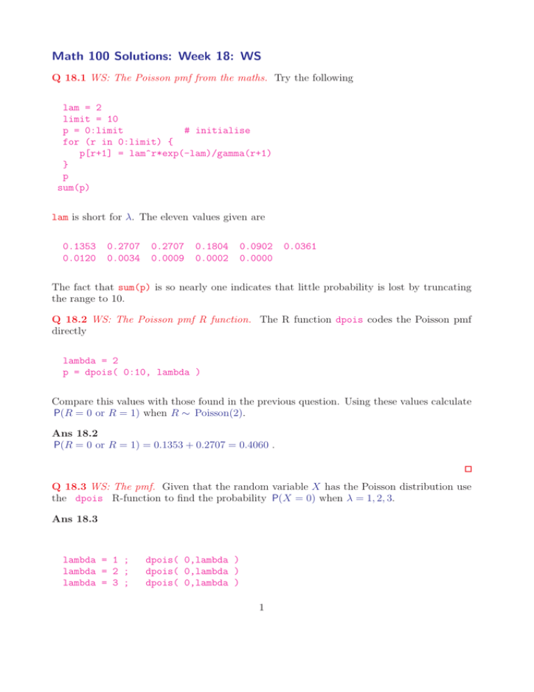
Q 18.1 WS: The Poisson pmf from the maths. Try the following
lam = 2
limit = 10
p = 0:limit
# initialise
for (r in 0:limit) {
p[r+1] = lam^r*exp(-lam)/gamma(r+1)
}
p
sum(p)
lam is short for λ. The eleven values given are
0.1353
0.0120
0.2707
0.0034
0.2707
0.0009
0.1804
0.0002
0.0902
0.0000
0.0361
The fact that sum(p) is so nearly one indicates that little probability is lost by truncating
the range to 10.
Q 18.2 WS: The Poisson pmf R function. The R function dpois codes the Poisson pmf
directly
lambda = 2
p = dpois( 0:10, lambda )
Compare this values with those found in the previous question. Using these values calculate
P(R = 0 or R = 1) when R ∼ Poisson(2).
Ans 18.2
P(R = 0 or R = 1) = 0.1353 + 0.2707 = 0.4060 .
Q 18.3 WS: The pmf. Given that the random variable X has the Poisson distribution use
the dpois R-function to find the probability P(X = 0) when λ = 1, 2, 3.
Ans 18.3
lambda = 1 ;
lambda = 2 ;
lambda = 3 ;
dpois( 0,lambda )
dpois( 0,lambda )
dpois( 0,lambda )
1
The probs are 0.3679, 0.1353, 0.0498, and are decreasing.
When plotting you sometimes want to see multiple graphs next to each other. We can do
this by splitting the graphics window into subplots using the par and mfrow commands. The
command par(mfrow=c(r,c)) splits the graphics window into r rows and c columns. Try
this out in the next question.
Q 18.4 WS: The Poisson mean. Here are two Poisson pmfs.
par(mfrow=c(1,2))
# sets up subplots
barplot( dpois(0:10, lambda=1 ), names.arg=0:10, ylim=c(0,.4))
barplot( dpois(0:10, lambda=3 ), names.arg=0:10, ylim=c(0,.4))
The names.arg option is a vector of names to be plotted below each bar in the plot. The
ylim option takes a vector of length two that gives the range (min and max values) that the
y variable should be plotted over. Make sketches of the plots in your notes. On the sketches
indicate where the mean (expected value) should be and state which pmf has the greater
mean.
Ans 18.4
The second pmf with λ = 3.
Q 18.5 WS: Cumulative probabilities. The random variable R has the Poisson(3) distribution. Use the dpois R-function to find the probability P(X = 0), P(X = 1) and P(X = 2).
Sum these three values together to get P(X = 0 or 1 or 2). For cumulative probabilities we
could use the dpois function and sum them up or we could use the ppois function that
calculates it automatically.
lambda = 3 ;
ppois( 2, lambda )
Now find this probability when λ = 2 and when λ = 3.
Now find P(X > 5) for these values of λ. Do these increase?
Ans 18.5
lambda = 1 ;
lambda = 2 ;
lambda = 3 ;
ppois( 2, lambda )
ppois( 2, lambda )
ppois( 2, lambda )
The probs are 0.92, 0.68, 0.42, and are decreasing.
2
lambda = 1 ;
lambda = 2 ;
lambda = 3 ;
1-ppois( 5, lambda )
1-ppois( 5, lambda )
1-ppois( 5, lambda )
These increase.
Q 18.6 WS: Simulating Poisson random variables As with the Binomial distribution last
week we can simulate Poisson random variables using the rpois function. It takes two
parameters, n, the number of random variables you want to simulate and lambda, that
specifies the specific Poisson distribution to simulate from.
To simulate five Poisson(λ) random variables:
x = rpois(n=5,2)
x
x = rpois(5,10)
x
Now simulate 50 values from a Poisson(3) random variable and plot them.
x = rpois(50, 3)
hist(x)
Repeat this with more random variables (try n=100,500,1000). What is happening as you
increase n? Try with different values of λ as well.
Q 18.7 WS: Empirical Poisson Probabilities Simulate 1,000 Poisson(3) random variables
and find empirical estimates of P(X = 0), P(X = 1), P(X = 2) and P(X = 0 or 1 or 2).
x=rpois(1000,3)
sum(x==0)/1000
sum(x==1)/1000
sum(x==2)/1000
sum(x<=2)/1000
Compare these with the true values you found previously.
Q 18.8 WS: Large number convergence: Poisson to Normal. As the value of lambda increases, the Poisson distribution gets closer and closer to a Normal distribution (don’t worry
you will learn about this distribution in Math105). We can see this by using simulations of
Poisson random variables. Simulate 1,000 Poisson random variables with λ = 1, 10, 100, see
how the distribution becomes more centred and bell-shaped as λ increases.
3
x=rpois(1000,1)
hist(x)
Q 18.9 WS: Poisson to Normal using theoretical probabilities We can show the same thing
using the theoretical properties of the Poisson distribution. A reasonable range to plot the
Poisson pmf over is
range = 0:10
p = dpois(0:10, lambda=5 )
barplot( p, names.arg=0:10, ylim=c(0,.4))
Find a suitable range to plot Poisson pmfs for λ = 1, 10, 100. Plot. Can you see the same
shapes as you saw with the simulations?
Ans 18.9
√
Range: 10, 25 and 160. In fact the appropriate range grows as a function of λ. The
emerging shape is bell-shaped.
par( mfrow=c(2,2))
barplot( dpois(0:10,
barplot( dpois(0:10,
barplot( dpois(30:70,
barplot( dpois(70:130,
lambda=1 ),
lambda=5 ),
lambda=50 ),
lambda=100),
names.arg=0:10,
names.arg=0:10,
names.arg=30:70,
names.arg=70:130,
Q 18.10 WS: Rare events convergence: Binomial to Poisson.
converges to the Poisson(λ) pmf if
ylim=c(0,.4))
ylim=c(0,.4))
ylim=c(0,.4))
ylim=c(0,.4))
The Binomial(n, θ) pmf
n increases to ∞, and θ decreases to 0,
and such that the Binomial mean nθ = λ is constant.
Set λ = 2. We need to choose n and θ such that nθ = 2.
par(mfrow=c(3,2))
barplot( dbinom(0:20,size= 5,prob=2/5 ), names.arg=0:20,ylim=c(0,.4))
barplot( dbinom(0:20,size=10,prob=1/5 ), names.arg=0:20,ylim=c(0,.4))
barplot( dbinom(0:20,size=20,prob=1/10 ),names.arg=0:20,ylim=c(0,.4))
barplot( dpois(0:20,lambda=2 ), names.arg=0:20,ylim=c(0,.4),col=’yellow’)
Note 5 × 2/5 = 2, 10 × 1/5 = 2.
The last two plots are the closest.
4
Try with n = 40. Does it lie in between these?
Now repeat with λ = 4 and setting n and θ appropriately.
Lab100 Quiz Week 18
5