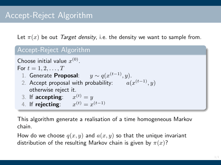
Accept-Reject Algorithm
Let π(x) be out Target density, i.e. the density we want to sample from.
Accept-Reject Algorithm
Choose initial value x(0) .
For t = 1, 2, . . . , T
1. Generate Proposal:
y ∼ q(x(t−1) , y).
2. Accept proposal with probability:
a(x(t−1) , y)
otherwise reject it.
3. If accepting: x(t) = y
4. If rejecting:
x(t) = x(t−1)
This algorithm generate a realisation of a time homogeneous Markov
chain.
How do we choose q(x, y) and a(x, y) so that the unique invariant
distribution of the resulting Markov chain is given by π(x)?
1/1
The Metropolis-Hastings algorithm
How to choose q(x, y) and a(x, y)?
One choice leads to the Metropolis-Hasting algorithm. The user specifies
a proposal kernel q(x, y). The algorithm then “automatically” chooses
the correct acceptance probability.
Metropolis-Hastings algorithm
Choose any proposal kernel q(x, y)
Define the Hastings ratio
H(x, y) =
π(y)q(y, x)
,
π(x)q(x, y)
where H(x, y) = ∞ if π(x)a(x, y) = 0.
The acceptance probability is
a(x, y) = min {1, H(x, y)} .
2/1
The Metropolis algorithm
A special case of the MH-algorithm is when the proposal kernel is
symmetric:
q(x, y) = q(y, x)
In this case the Hastings-ratio simplifies to
H(x, y) =
π(y)
π(y)q(y, x)
=
.
π(x)q(x, y)
π(x)
Example: The most common example, is when the proposal is normal
distributed with x as the mean value, and τp as the precision:
r
τp
1
exp − τp (y − x)2 .
q(x, y) =
2π
2
Clearly, q(x, y) = q(y, x).
3/1
Burn-in
Generate X (0) ∼ π0 (x), an initial distribution, typically different
from π(x).
Create irreducible Markov chain X (0) , X (1) , X (2) , . . . with π(x) as
invariant distribution.
For small values of t the distribution of X (t) can be quite different
from π(x).
As a consequence, the sample mean
T
1 X (t)
X
T t=1
is biased, i.e. E
h P
T
1
Instead consider
T
t=1
i
6 µ.
X (t) =
T
1 X (m+t)
X
,
T t=1
where m is the length of the burn-in
4/1
The effect of burn-in
0.0
−15
0.2
−5
0
0.4
Histogram of x[1:200]
100
200
300
400
500
−15
−10
−5
0
Histogram of x
0.0
−15
0.2
−5
0
0.4
0
100
200
300
400
500
−15
−10
−5
0
Histogram of x[s]
0.0
−15
0.2
−5
0
0.4
0
0
100
200
300
400
500
−15
−10
−5
0
5/1
Variance of the sample mean: IID Case
Assume we have independent samples X (1) , X (2) , . . . , X (T ) from π(x).
Assume E[X (t) ] = µ and V ar[X (t) ] = σ 2 .
The sample mean is
T
1 X (t)
X
T t=1
For the sample mean we have the following results.
#
"
T
1 X (t)
X
=µ
E
T t=1
"
#
T
1 X (t)
1
Var
X
= σ2
T t=1
T
"
#
T
1 X (t)
T · Var
X
= σ2 .
T t=1
6/1
Variance of the sample mean: Markov Chain Case
Assume X (1) , X (2) , X (3) , . . . is an irreducible Markov chain with
invariant distribution with density π(x).
Further, assume that X (1) ∼ π(x) which implies that X (t) ∼ π(X) for all
t = 2, 3, 4, . . ., which in turn implies that E[X (t) ] = µ and
Var[X (t) ] = σ 2 .
The expected value of the sample mean is (again)
#
"
T
1 X (t)
X
= µ.
E
T t=1
So the expected value of the sample mean is unaffected by the shift from
IID sample to Markov chain.
7/1
Variance of the sample mean: Markov Chain Case
Regarding the variance we have
#
"
T
1 X (t)
X
→ σ2
T · Var
T t=1
1+2
∞
X
i=1
ρi
!
,
where
ρi = Corr(X
(t)
,X
(t+i)
E (X (t) − µ)(X (t+i) − µ)
)=
σ2
is the lag-i auto-correlation.
P∞
We call σ 2 (1 + 2 i=1 ρi ) the asymptotic variance.
P∞
Trying to get τ = 1 + 2 i=1 ρi to be as small as possible seems like
a good idea.
If we just want to estimate µ this is a brilliant idea.
8/1
Tuning
Assume the proposal kernel is
r
τp
1
2
q(x, y) =
exp − τp (y − x) .
2π
2
Now, τp is an “algorithm parameter” that we need to choose.
What is a good choice of τp ? This is an example of tuning an algorithm.
Example: Assume target density is normal
r
τ
1
π(x) =
exp(− x2 )
2π
2
The optimal choice (in terms of reducing the asymptotic variance) is so
that the acceptance probability is around 40%.
If π(x1 , x2 , . . . , xk ) is multivariate normal, the optimal choice of τp
corresponds to an acceptance probability of 0.234.
9/1
Tuning, Acceptance probability and Auto-correlation
Series x$x
Histogram of x$x
−1.5
1.0
0.6
0.4
0.0
0.0
0.2
0.5
−0.5
1.0
0.8
0.5 1.0
1.5
acceptance prob.: 0.024
0
50
100
150
200
250
−1.5 −1.0 −0.5
0.0
0.5
1.0
1.5
100
150
200
250
20 x$x
Series
30
40
1.0
1
2
0.0 0.2 0.4 0.6 0.8 1.0
0.30
3
0.20
0.10
0.00
200
10
0.6
0
2
1
150
0
0.4
−1
0
−1
100
40
Histogram of x$x
−2
50
30
0.0
−2
acceptance prob.: 0.8
0
20 x$x
Series
0.2
0.2
0.1
0.0
50
10
0.8
0.5
0.4
0.3
1
0
−1
−2
0
0
Histogram of x$x
2
acceptance prob.: 0.22
250
−2
−1
0
1
2
3
0
5
10
15
20
25
30
10/1
A bivariate case example
0.99 1
1
Target: N (0, 0),
0.99
Gibbs sampling
3
0
−2
−3
−2
−2
−1
−1
−1
0
0
1
1
1
2
2
2
Acceptance prob.: 1
1
2
−2
−1
0
1
2
−1
0
1
2
0.8
2
−3
0.0
−2
0.2
−1
0.4
0
0.6
1
2
1
−3
−2
−1
0
−2
1.0
0
3
−1
3
−2
0
500
1000
1500
2000
2500
0
500
1000
1500
2000
2500
0
5
10
15
20
25
30
11/1
A bivariate case example
1
0.99 Target: N (0, 0),
0.99
1
100
0
Proposal covariance
0
100
Acceptance prob.: 0.0016
3
0
−2
−3
−2
−2
−1
−1
−1
0
0
1
1
1
2
2
2
−1
0
1
2
−2
−1
0
1
2
−3
−2
0
5
−1
0
1
2
3
0.8
0.6
0.2
0.0
0.0
0.0
0.5
0.5
0.4
1.0
1.0
1.5
1.5
1.0
−2
0
500
1000
1500
2000
2500
0
500
1000
1500
2000
2500
10
15
20
25
30
12/1
A bivariate case example
1
0.99 Target: N (0, 0),
0.99
1
1 0
Proposal covariance:
0 1
Acceptance prob.: 0.1196
3
0
−2
−3
−2
−2
−1
−1
−1
0
0
1
1
1
2
2
2
0
1
2
−2
−1
0
1
2
−3
−2
0
5
−1
0
1
2
3
0
500
1000
1500
2000
2500
0.4
0.2
0.0
−2
−2
−1
−1
0
0
0.6
1
1
0.8
2
1.0
−1
2
−2
0
500
1000
1500
2000
2500
10
15
20
25
30
13/1
A bivariate case example
1
0.99 Target: N (0, 0),
0.99
1
0.01
0
Proposal covariance:
0
0.01
Acceptance prob.: 0.6892
3
0
−2
−3
−2
−2
−1
−1
−1
0
0
1
1
1
2
2
2
−1
0
1
2
−2
−1
0
1
2
−3
−2
0
5
−1
0
1
2
3
0
500
1000
1500
2000
2500
0.8
0.0
−1.0
−0.5
0.2
0.0
0.4
0.5
1.0
0.6
1.5
2.0
1.0
−2
0
500
1000
1500
2000
2500
10
15
20
25
30
14/1
A bivariate case example
0.99 1
2
1
0.99
Proposal covariance: 2.38
2
0.99
1
1
Target: N (0, 0),
0.99
Acceptance prob.: 0.352
3
0
−2
−3
−2
−2
−1
−1
−1
0
0
1
1
1
2
2
2
1
2
−2
−1
0
1
2
−2
0
5
−1
0
1
2
3
0.8
2
−3
0.0
−2
0.2
−1
0.4
0
0.6
1
2
1
−3
−2
−1
0
−3
1.0
0
3
−1
3
−2
0
500
1000
1500
2000
2500
0
500
1000
1500
2000
2500
10
15
20
25
30
15/1
Optimum proposal
Assume target is a d-dimensional normal:
π(x) = Nd (µ, Σ)
and the proposal is normal:
q(x, y) = Nd (x, Σq )
Then the optimum choice of proposal variance Σq is
Σq =
2.382
Σ
d
Catch: Σ is unknown.
Solutions: Pilot run or adaptive MCMC.
16/1
Reminder: The Gibbs sampler
Aim: We want to sample θ = (θ1 , θ2 , . . . , θk ) from a pdf/pf π(θ).
Assume θi ∈ Ωi ⊆ Rdi . Then, θ ∈ Ω1 × Ω2 × · · · × Ωk ⊆ Rd1 +d2 +···+dk
We can now (under some conditions) generate an approximate sample
from π(θ) as follows:
Gibbs Sampler
(0)
(0)
(0)
Choose initial value θ (0) = (θ1 , θ2 , . . . , θk ).
For t = 1, 2, . . . , T
◮
For i = 1, 2, . . . , k
(t)
1. Generate θi
(t)
(t)
(t−1)
(t−1)
∼ π(θi |θ1 , . . . , θi−1 , θi+1 , . . . , θk
)
Question: What if we cannot generate samples from one or more of the
full conditional distributions?
Solution: Use a Metropolis-Hastings update instead!
17/1
Metropolis within Gibbs (MwG)
Gibbs Sampler
(0)
(0)
(0)
Choose initial value θ (0) = (θ1 , θ2 , . . . , θk ).
For t = 1, 2, . . . , T
◮
For i = 1, 2, . . . , k
(t)
(t)
(t−1)
1. Generate proposal θi′ ∼ q(θi′ |θ1 , . . . , θi−1 , θi
2. Calculate Hastings ratio
(t)
(t−1)
H(θi
, θi′ ) =
(t)
(t−1)
(t−1)
, . . . , θk
(t−1)
π(θi′ |θ1 , . . . , θi−1 , θi+1 , . . . , θk
)
)
(t−1)
(t−1)
(t−1) (t)
(t)
π(θi
|θ1 , . . . , θi−1 , θi+1 , . . . , θk
)
×
(t−1)
(t)
(t)
(t−1)
|θ1 , . . . , θi−1 , θi′ , . . . , θk
)
(t)
(t)
(t−1)
(t−1)
q(θi′ |θ1 , . . . , θi−1 , θi
, . . . , θk
)
q(θi
3. With probability
n
o
(t−1) ′
min 1, H(θi
, θi )
(t)
set θi
(t)
= θi′ (accept) otherwise set θi
(t−1)
= θi
(reject).
18/1
Metropolis within Gibbs: Comments
Notice that each of the k component updates have π(θ) as their
invariant distribution.
Hence the MwG algorithm has π(θ) as its invariant distribution.
Irreducibility is not automatically fulfilled.
Special case: Assume that q(θi |θ−i ) is given by the full conditional:
(t)
(t)
(t−1)
(t−1)
q(θi′ |θ1 , . . . , θi , θi+1 , . . . , θk
=
(t−1)
Then H(θi
)
(t)
(t)
(t−1)
(t−1)
π(θi′ |θ1 , . . . , θi−1 , θi+1 , . . . , θk
).
, θi′ ) = 1, hence all proposals are accepted.
In fact, this is exactly the usual Gibbs sampler!
19/1
Prior predictions
Predicting future observations without data.
Notation: Let x̃ denote a prediction.
Assume:
Data model:
x̃|θ ∼ π(x|θ)
Prior:
π(θ)
The above assumptions implies a joint distribution of data, x, and
parameter, θ:
π(x, θ) = π(x|θ)π(θ).
We are interested in predicting a future observation, i.e. the (marginal)
distribution of x, i.e. when ignoring θ, i.e.
x̃ ∼ π(x),
where
π(x) =
Z
π(x|θ)π(θ)dθ.
20/1
Prior prediction: Normal case, τ known
Assume:
Data model: π(x|µ) ∼ N (µ, τ ).
Prior:
π(µ) = N (µ0 , τ0 )
Prior predictive distribution
Z
π(x) = π(x|µ)π(µ)dµ
r
Z r
1
1
τ
τ0
2
2
exp − τ (x − µ)
exp − τ0 (µ − µ0 ) dµ
=
2π
2
2π
2
r
τ τ0 1
1 τ τ0
=
exp −
(x − µ0 )2
τ + τ0 2π
2 τ + τ0
τ τ0
= N µ0 ,
.
τ + τ0
21/1
dnorm(x.seq, mu0, 1/sqrt(tau0))
Prior predictive distribution
0.10
Prior
Prior predictive
Predictive if µ =170
0.08
0.06
0.04
0.02
0.00
140
150
160
170
180
190
200
22/1
Simulating the prior predictive distribution
If π(x) is difficult to derive or not easily simulated from directly we can
use another strategy.
Simulating the prior predictive distribution can be done as follows:
1. Generate parameter from prior:
2. Conditional on θ generate x:
θ ∼ π(θ)
x̃ ∼ π(x|θ)
Now x̃ is a sample from the prior predictive distribution.
23/1
Posterior prediction
Predicting future observation given data.
Assume:
Data model:
x|θ ∼ π(x|θ)
Prior:
π(θ)
The joint distribution of predicted data x̃, data x and parameter θ is
π(x̃, x, θ) = π(x̃|θ)π(x|θ)π(θ)
∝ π(x̃|θ)π(θ|x).
Notice: Here π(x̃|θ) and π(x|θ) represent the same distribution.
The posterior predictive distribution is the (marginal) distribution of x̃
conditional on data x:
Z
Z
Z
π(x̃, θ, x)
dθ ∝ π(x̃|θ)π(x|θ)π(θ)dθ
π(x̃|x) = π(x̃, θ|x)dθ =
π(x)
Z
∝ π(x̃|θ)π(θ|x)dθ
24/1
Hence, the posterior acts as a prior for the predictions.
Posterior prediction: Normal case, τ known
iid
Data model: X1 , X2 , . . . , Xn ∼ N (µ, τ ).
Prior: π(µ) = N (µ0 , σ0 ).
x̄+τ0 µ0
Posterior: π(µ|x) = N nτnτ
+τ0 , nτ + τ0 .
Recall that the prior prediction (of one observation) was
τ0 τ
x̃ ∼ N µ0 ,
τ + τ0
Since the posterior is the “prior” for the posterior prediction we have
nτ x̄ + τ0 µ0 (nτ + τ0 )τ
,
x̃|x ∼ N
nτ + τ0
τ + nτ + τ0
When n is large we have x̃|x
approx
∼
N (x̄, τ ).
25/1
dnorm(x.seq, mu0, 1/sqrt(tau0))
dnorm(x.seq, mu0, 1/sqrt(tau0))
Prior and posterior predictive distributions
0.10
Prior
Prior predictive
Predictive if µ =170
0.08
0.06
0.04
0.02
0.00
140
0.10
150
160
170
180
190
200
170
180
190
200
Posterior
Prior predictive
Posterior predictive
0.08
0.06
0.04
0.02
0.00
140
150
160
26/1
Posterior prediction using a graph
27/1
Model checking
Idea: If the model is correct posterior predictions of the data should look
similar to the observed data.
Difficulty: Who to choose a good measure of “similarity”.
Example: We have observed a sequence of n = 20 zeros and ones:
11000001111100000000
Model: X1 , X2 , . . . , X20 are IID and P (Xi = 1) = p.
Prior: π(π) = Be(α, β).
Posterior: π(π|x) = Be(#1 + α, #0 + β).
Model checking: We simulate posterior predictive realisations
X̃(1) , X̃(2) , . . . , X̃(N ) , where
(i)
(i)
(n)
X̃(i) = (X1 , X2 , . . . , X2 ).
If these vectors look “similar” to the data above, the model is probably
ok.
28/1
Model checking: First attempt (A failure)
Define summary function
s(x) = Number of ones in the sequence x
Histogram for s(x̃(i) ) for N = 10, 000 independent posterior predictions:
0
400
800
1400
Histogram of proportion of ones
0.0
0.2
0.4
0.6
0.8
Clearly the observed number of ones is in no way unusual compared to
the posterior predictions.
This is really expected — so we need another summary function s(x).
29/1
Model checking: Second attempt (A success)
Define summary function
s(x) = Number of switches between ones and zeros in x
In the data the number of switches is 3:
11000001111100000000
Histogram for s(x̃(i) ) for N = 10, 000 independent posterior predictions:
0
500 1000
Histogram of number of switches
0
5
10
15
20
Only around 1.7% of the posterior prediction have 3 or fewer switches.
This suggests that the model assumption of independence is questionable.
30/1