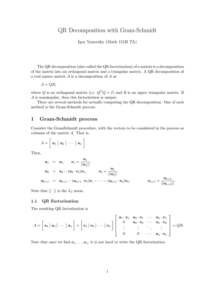
QR Decomposition with Gram-Schmidt
Igor Yanovsky (Math 151B TA)
The QR decomposition (also called the QR factorization) of a matrix is a decomposition
of the matrix into an orthogonal matrix and a triangular matrix. A QR decomposition of
a real square matrix A is a decomposition of A as
A = QR,
where Q is an orthogonal matrix (i.e. QT Q = I) and R is an upper triangular matrix. If
A is nonsingular, then this factorization is unique.
There are several methods for actually computing the QR decomposition. One of such
method is the Gram-Schmidt process.
1
Gram-Schmidt process
Consider the GramSchmidt procedure, with the vectors to be considered in the process as
columns of the matrix A. That is,
·
¸
¯
¯
¯
¯
¯
¯
A = a1 a2 · · · an .
Then,
u1 = a1 ,
e1 =
u1
,
||u1 ||
u2 = a2 − (a2 · e1 )e1 ,
e2 =
u2
.
||u2 ||
uk+1 = ak+1 − (ak+1 · e1 )e1 − · · · − (ak+1 · ek )ek ,
ek+1 =
uk+1
.
||uk+1 ||
Note that || · || is the L2 norm.
1.1
QR Factorization
The resulting QR factorization is

·
A=
¯ ¯
¯
a1 ¯ a2 ¯ · · · ¯ an
¸
·
=
¸
¯ ¯
¯

¯
¯
¯
e1 e2 · · · en 

a1 · e1 a2 · e1 · · ·
0
a2 · e2 · · ·
..
..
..
.
.
.
0
0
···
an · e1
an · e2
..
.
an · en
Note that once we find e1 , . . . , en , it is not hard to write the QR factorization.
1



 = QR.

2
Example
Consider the matrix


1 1 0
A =  1 0 1 ,
0 1 1
with the vectors a1 = (1, 1, 0)T , a2 = (1, 0, 1)T , a3 = (0, 1, 1)T .
Note that all the vectors considered above and below are column vectors. From now on,
I will drop T notation for simplicity, but we have to remember that all the vectors are
column vectors.
Performing the Gram-Schmidt procedure, we obtain:
u1 = a1 = (1, 1, 0),
µ
¶
u1
1
1 1
e1 =
= √ (1, 1, 0) = √ , √ , 0 ,
||u1 ||
2
2 2
¶
µ
¶ µ
1
1 1
1 1
,− ,1 ,
u2 = a2 − (a2 · e1 )e1 = (1, 0, 1) − √ √ , √ , 0 =
2 2
2
2 2
µ
¶ µ
¶
u2
1 1
1
1
1 2
e2 =
=p
, − , 1 = √ , −√ , √ ,
||u2 ||
6
6 6
3/2 2 2
u3 = a3 − (a3 · e1 )e1 − (a3 · e2 )e2
µ
¶
µ
¶ µ
¶
1 1
1
1
1 2
1 1 1
1
√
√
√
√
√
√
√
√
√
√
,
,0 −
,−
,
= −
,
,
,
= (0, 1, 1) −
2
2 2
6
6
6 6
3 3 3
µ
¶
u3
1 1 1
e3 =
= −√ ,√ ,√ .
||u3 ||
3 3 3
Thus,
·
Q =

¯
¯
¯
e1 ¯ e2 ¯ · · · ¯ en
¸


=
√1
2
√1
2
0

√1
6
− √16
√2
6
 2
√
2
a1 · e1 a2 · e1 a3 · e1

0
a2 · e2 a3 · e2  =  0
R = 
0
0
a3 · e3
0
2
− √13


√1
,
3 
√1
3
√1
√1
2
2
√3
√1
6
6
0 √23


.