Numerical Optimization!
Robert Stengel!
Robotics and Intelligent Systems MAE
345, Princeton University, 2015
•! Gradient search
•! Gradient-free search
•!
•!
•!
•!
–! Grid-based search
–! Random search
–! Downhill simplex method
Monte Carlo evaluation
Simulated annealing
Genetic algorithms
Particle swarm optimization
Copyright 2015 by Robert Stengel. All rights reserved. For educational use only.
http://www.princeton.edu/~stengel/MAE345.html
1
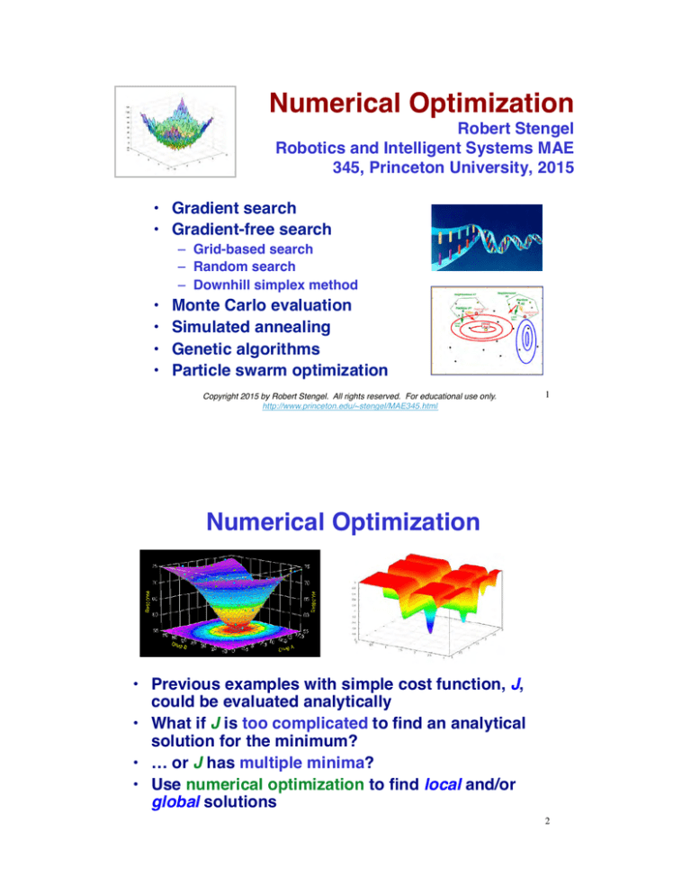
Numerical Optimization
•! Previous examples with simple cost function, J,
could be evaluated analytically
•! What if J is too complicated to find an analytical
solution for the minimum?
•! … or J has multiple minima?
•! Use numerical optimization to find local and/or
global solutions
2
Two Approaches to
Numerical Minimization
1)" Slope and curvature of surface
a)" Evaluate gradient , !J/!u, and search for zero
b)" Evaluate Hessian, !2J/!u2, and search for positive value
!J
"!J%
= starting guess
$# '& =
! u o ! u u=u0
!J
"!J%
"!J%
"!J%
such that
$# '& = $# '& + ) $# '& =
!u n
! u n(1
! u n ! u u=un
… until gradient is
close enough to zero
!J
!J
<
! u n ! u n(1
2) Evaluate cost, J , and search for smallest value
J o = J ( u o ) = starting guess
J1 = J o + !J1 ( u o + !u1 ) such that
J 2 = J1 + !J 2 ( u1 + !u 2 ) such that
J1 < J o
J 2 < J1
Stop when difference
between Jn and Jn–1
is negligible
3
Gradient/Hessian Search to
Minimize a Quadratic Function
Cost function, gradient,
and Hessian matrix
J=
=
1
( u ! u *)T R ( u ! u *) , R > 0
2
1 T
( u Ru ! uT Ru * !u *T Ru + u *T Ru *)
2
"J
T
= ( u ! u *) R = 0 when u = u *
"u
"2J
= R = symmetric constant > 0
" u2
Guess a starting value
of u, uo
2
!J
T
T ! J
= ( u o " u *) R = ( u o " u *)
! u u=uo
! u2
!J
( uo " u *)T = ! u
u=uo
R "1
u=uo
( row )
Solve for u*
#" J
&
u* = u o ! R %
(
%$ " u u=uo ('
!1
T
( column )
4
Optimal Value of Quadratic
Function Found in a One Step
#" J
&
u* = u o ! R %
(
%$ " u u=uo ('
T
!1
#" 2 J
= uo ! % 2
%$ " u
!1
& #" J
&
( %
(
u=uo (
' %$ " u u=uo ('
T
•! Gradient establishes general
search direction
•! Hessian fine-tunes direction
and tells exactly how far to go
5
Numerical Example
•! Cost function and derivatives
J=
T
.
2
1 0 (! u1 $ ! 1 $ + ( 1 2 + (! u1 $ ! 1 $ + 0
*
*
'
'
&
&
/ #
3
*
- #
2 0 *#" u2 &% #" 3 &% - ) 2 9 , *#" u2 &% #" 3 &% - 0
,
)
,4
1)
T
T
(! u $ !
+
( 1 2 +
! 5J $
1
1 $- ( 1 2 +
& '#
*
-; R = *
#" &% = *##
&
5u
*" u2 &% " 3 % - ) 2 9 ,
) 2 9 ,
)
,
•! First guess at optimal control
•! Solution from starting
point
#"J
u* = u o ! R %
%$ " u
!1
! u1 $
! 4 $
#
& =#
#" u2 &%
" 7 &%
0
•! Derivatives at starting point
T
)" 4 % " 1 % , )
!J
= +$
(
. +
! u u=u0 +*# 7 '& $# 3 '& .- *
) 1 2
R=+
* 2 9
1 2 , " 11 %
.=
2 9 - $# 42 '&
,
.
-
&
(
u= uo (
'
T
*
! u1 $ ! 4 $ ( 9 / 5 '2 / 5 + ! 11 $
u* = #
'
& =
#" u2 &% #" 7 &% *) '2 / 5 1 / 5 -, #" 42 &%
! 4 $ ! 3 $ ! 1 $
=#
'
=
" 7 &% #" 4 &% #" 3 &%
6
Newton-Raphson
Iteration
•! Many cost functions are not quadratic
•! However, the surface is well-approximated by a
quadratic in the vicinity of the optimum, u*
J ( u * +!u ) " J ( u *) + !J ( u *) + ! 2 J ( u *) + ...
!J ( u *) = !uT
#J
=0
# u u=u*
$# 2 J
! J ( u *) = !u & 2
%# u
2
T
'
) !u * 0
u=u* (
Optimal solution requires multiple steps
7
Newton-Raphson Iteration
Newton-Raphson algorithm is an iterative search
using both the gradient and the Hessian matrix
#"2J
u k +1 = u k ! % 2
%$ " u
&
(
u= u k (
'
!1
#"J
%
%$ " u
&
(
u= u k (
'
T
8
Difficulties with NewtonRaphson Iteration
#"2J
u k +1 = u k ! % 2
%$ " u
!1
& #"J
( %
"u
u= u k (
' %$
&
(
u= u k (
'
T
•! Good when close to the optimum, but …
•! Hessian matrix (i.e., the curvature) may be
–! Hard to estimate, e.g., large effects of
small errors
–! Locally misleading, e.g., wrong curvature
•! Gradient searches focus on local minima
9
Steepest-Descent Algorithm Multiplies
Gradient by a Scalar Constant
$#J
u k +1 = u k ! " &
&% # u
'
)
u= u k )
(
T
•! Replace Hessian matrix
by a scalar constant
•! Gradient is orthogonal to
equal-cost contours
10
Choice of SteepestDescent Constant
If gain is too small
Convergence is slow
If gain is too large
Convergence oscillates or
may fail
Solution: Make gain adaptive
11
Optimal Steepest-Descent Constant
•! Use optimal gain on each
iteration
•! Find optimal step size by
evaluating cost, J, for
intermediate solutions (with
same dJ/du)
•! Adjustment rule (partial) for
–!
–!
–!
–!
Starting estimate, Jo
1st estimate, J1, using "
2nd estimate, J2, using 2"
If J2 > J1
•! Quadratic fit through 3 points
to find best " and use for next
iteration
–! Else
•! 3rd estimate using 4"
•! etc.
12
Gradient Search
Issues
Newton Raphson
Steepest Descent
$# J
'
u k+1 = u k ! " &
)
&% # u u=uk )(
T
#" 2 J
u k+1 = u k ! % 2
%$ " u
!1
& #" J
&
( %
(
"
u
%
('
u=u
u=u k (
$
k
'
T
•! Need to evaluate gradient (and possibly Hessian matrix)
•! Not global: gradient searches focus on local minima
•! Convergence may be difficult with noisy
or complex
cost functions
13
Gradient-Free Search:
Grid-Based Search
J o = J ( u o ) = starting guess
J1 = J o + !J1 ( u o + !u1 ) such that
J 2 = J1 + !J 2 ( u1 + !u 2 ) such that
J1 < J o
J 2 < J1
14
Gradient-Free Search:
Random Search
J o = J ( u o ) = starting guess
J1 = J o + !J1 ( u o + !u1 ) such that
J 2 = J1 + !J 2 ( u1 + !u 2 ) such that
J1 < J o
J 2 < J1
* Select control parameters using a
random number generator
15
Three-Parameter Grid Search
n = 125
n = 1000
•! Regular spacing
•! Fixed resolution
•! Trials grow as mn, where
–! n = Number of parameters
–! m = Resolution
16
Three-Parameter Random
Field Search
n = 125
n = 1000
Variable spacing and resolution
Arbitrary number of trials
Random space-filling
17
Directed (Structured) Search
for Minimum Cost
Continuation of grid-based or random search
Localize areas of low cost
Increase sampling density in those areas
18
•!
Directed (Structured) Search
for Minimum Cost
Interpolate or extrapolate from one or more starting points
19
Downhill Simplex Search
(Nelder-Mead Algorithm)
•! Simplex: N-dimensional figure in control space defined by
–! N + 1 vertices
–! (N + 1) N / 2 straight edges between vertices
20
Search Procedure for
Downhill Simplex Method
•! Select starting set of
vertices
•! Evaluate cost at each vertex
•! Determine vertex with
largest cost (e.g., J1 at right)
•! Project search from this vertex through middle of
opposite face (or edge for N = 2)
•! Evaluate cost at new vertex (e.g., J4 at right)
•! Drop J1 vertex, and form simplex with new vertex
•! Repeat until cost is small
Humanoid Walker optimized via Nelder-Mead
http://www.youtube.com/watch?v=BcYPLR_j5dg
21
Monte Carlo Evaluation of
Systems and Cost Functions
•! Multiple evaluations of a function with
uncertain parameters using
–! Random number generators, and
–! Assumed or measured statistics of parameters
•! Not an exhaustive evaluation of all parameters
22
Monte Carlo Evaluation of
Systems and Cost Functions
•!
•!
Example: 2-D quadratic function with added
Gaussian noise
Each trial generates a different result (! z = 4 )
[X,Y] = meshgrid(-8:.5:8);
Z = X.^2 + Y.^2;
Z1 = Z + 4*randn(33);
surf(X,Y,Z1)
colormap hsv
alpha(.4)
23
[X,Y] = meshgrid(-8:.5:8);
Z = X.^2 + Y.^2;
Z1 = Z + 4*randn(33);
surf(X,Y,Z1)
colormap hsv
alpha(.4)
Effect of Increasing
Noise on Cost Function
!z = 0
!z = 8
!z = 4
! z = 16
24
Iso-Cost Contours Lose Structure
with Increasing Noise
!z = 0
!z = 8
!z = 4
! z = 16
25
Effect of Averaging on
Noisy Cost Function
•! One trial
!z = 0
•! One trial ! z = 16
[X,Y] = meshgrid(-8:.5:8);
Z = X.^2 + Y.^2;
Z1 = Z + 16*randn(33);
Z2 = Z1;
% Averaged Z1
for k = 1:1000
Z1 = Z + 16*randn(33);
Z2 = Z1 * (1/(k + 1)) + Z2 * (k/(k+1));
end
figure
surf(X,Y,Z2)
colormap hsv
alpha(.4)
•! 1,000 trials ! z = 16
26
Estimating the
Probability of Coin Flips
% Single coin
x
= [];
prob = round(rand);
for k = 1:20000
prob = round(rand) * (1/(k + 1)) + prob * (k/(k+1));
x
= [x prob];
end
figure
plot(x), grid
•! Single coin
–! Exhaustive search: Correct answer in
2 trials
–! Random search (20,000 trials)
% 21 coins
y
= [];
prob = round(rand);
for k = 1:20000
for j = 1:21
coin(j) = round(rand);
end
score = sum(coin);
if score > 10
result = 1;
else result = 0;
end
prob = result * (1/(k + 1)) + prob * (k/(k+1));
y
= [y prob];
end
figure
plot(y), grid
•! 21 coins
–! Exhaustive search: Correct answer in
nm = 221 = 2,097,152 trials
–! Random search (20,000 trials)
...
27
Random Search Excels When There
are Many Uncertain Parameters
•!
Single coin
–! Exhaustive search: Correct answer in 2
trials
–! Random search (20,000 trials)
•!
21 coins
–! Exhaustive search: Correct answer in
nm = 221 = 2,097,152 trials
–! Random search (20,000 trials)
28
•!
Physical Annealing
Produce a strong, hard object made of crystalline material
–! High temperature allows molecules to redistribute to relieve stress,
remove dislocations
–! Gradual cooling allows large, strong crystals to form
–! Low temperature working produces desired crystal structure and shape
Turbojet Engine
Turbines
Turbine Blade
Casting
Single-Crystal
Turbine Blade
29
Simulated Annealing Algorithm
•!
•!
•!
Goal: Find global minimum among local
minima
Approach: Randomized search, with
convergence that emulates physical annealing
–! Evaluate cost, Jk
–! Accept if Jk < Jk – 1
–! Accept with probability Pr(E) if Jk > Jk – 1
Probability distribution of energy state, E
(Boltzmann Distribution)
Pr(E) ! e" E / kT
k : Boltzmann's constant
T : Temperature
•!
Algorithm
s cooling schedule
accepts many bad
guesses at first, fewer as iteration number, k, increases
General Simulated Annealing Algorithm
http://www.mathworks.com/matlabcentral/fileexchange/10548-general-simulated-annealing-algorithm
30
Application of Annealing
Principle to Search
•! If cost decreases (J2 < J1), always
accept new point
•! If cost increases (J2 > J1), accept new
point with probability proportional to
Boltzmann factor
•!
•!
e! ( J2 ! J1 ) / kT
Occasional diversion from convergent path intended to prevent
entrapment by a local minimum
As search progresses, decrease kT, making probability of
accepting a cost increase smaller
Realistic Bird Flight Animation by SA
http://www.youtube.com/watch?v=SoM1nS3uSrY
SA Face Morphing
http://www.youtube.com/watch?v=SP3nQKnzexs
31
e! ( J2 ! J1 ) / kT
Combination of Simulated
Annealing with Downhill
Simplex Method
•! Introduce random wobble
to
simplex search
SA Mona Lisa
http://www.youtube.com/watch?v=eHWZcPLRMjQ
–! Add random components to costs
evaluated at vertices
–! Project new vertex as before
based on modified costs
–! With large T, this becomes a
random search
–! Decrease random components on
a cooling schedule
•! Same annealing strategy as before
–! If cost decreases (J2 < J1), always
accept new point
–! If cost increases (J2 > J1), accept
new point probabilistically
–! As search progresses, decrease T
J1SA = J1 + !J1 ( rng )
J 2SA = J 2 + !J 2 ( rng )
J 3SA = J 3 + !J 3 ( rng )
... = ...
32
Genetic Coding,
Recombination, and Mutation
33
Broad Characteristics
of Genetic Algorithms
•! Search based on the coding of a parameter set, not the
parameters themselves
•! Search evolves from a population of points
•! Blind
search, i.e., without gradient
•! Probabilistic transitions from one control state to another
•! Control parameters assembled as genes of a single
chromosome strand (Example: four 4-bit parameters)
34
Progression of a
Genetic Algorithm
Most fit chromosome evolves from a sequence
of reproduction, crossover, and mutation
•! Initialize algorithm with N (even)
random chromosomes, cn (two
8-bit genes or parameters in
example)
•! Evaluate fitness, Fn, of each
chromosome
•! Compute total fitness, Ftotal, of
chromosome population
N
Ftotal = ! Fn
F1
F2
F3
F4
Bigger F is better
n=1
35
Genetic Algorithm:
Reproduction
•! Reproduce N additional copies of the N
originals with probabilistic weighting
based on relative fitness, Fn /Ftotal, of
originals (Survival of the fittest)
•! Roulette wheel selection:
–! Pr(cn) = Fn /Ftotal
–! Multiple copies of most-fit chromosomes
–! No copies of least-fit chromosomes
1
2
3
4
5
6
7
8
9
10
11
12
13
14
15
16
17
18
19
20
21
22
23
24
Starting Set
Reproduced Set
36
1
2
3
4
5
6
7
8
9
10
11
12
13
14
15
16
17
18
19
20
21
22
23
24
Reproduction Eliminates
Least Fit Chromosomes
Probabilistically
Reproduced Set
Starting Set
37
Genetic Algorithm: Crossover
•!
Arrange N new chromosomes in N/2
pairs chosen at random
Head
Tail
•!
Interchange tails that are cut at
random locations
Head
Tail
38
Crossover Creates New
Chromosome Population Containing
Old Gene Sequences
Reproduced Set
Crossover Set
39
Genetic Algorithm: Mutation
Flip a bit, 0 -> 1 or 1 -> 0, at
random every 1,000 to 5,000 bits
Crossover Set
Mutated Set
40
Create New Generations By
Reproduction, Crossover, and Mutation
Until Solution Converges
Chromosomes narrow in on best
values with advancing generations
Fmax and Ftotal increase with
advancing generations
Open Genetic Algorithm Toolbox
http://www.mathworks.com/matlabcentral/fileexchange/37998-open-genetic-algorithm-toolbox
41
Comments on GA
1
2
3
4
5
6
7
8
9
10
11
12
13
14
15
16
17
18
19
20
21
22
23
24
GA Mona Lisa
http://www.youtube.com/watch?v=rGt3iMAJVT8
•! Short, fit genes tend to survive crossover
•! Random location of crossover
–! produces large and small variations in
genes
–! interchanges genes in chromosomes
•! Multiple copies of best genes evolve
•! Alternative implementations
–! Real numbers rather than binary numbers
–! Retention of elite
chromosomes
–! Clustering in fit
regions to produce elites
42
Particle Swarm
Optimization
•! Converse of the GA: Uses multiple cost evaluations to
guide parameter search directly
•! Stochastic, population-based algorithm
•! Search for optimizing parameters modeled on social
behavior of groups that possess cognitive consistency
•! Particles = Parameter vectors
•! Particles have position and velocity
•! Projection of own best (Local best)
•! Knowledge of swarm
s best
–! Neighborhood best
–! Global best
Peregrine Falcon Hunting Starlings in Rome
https://www.youtube.com/watch?v=V-mCuFYfJdI
43
Particle Swarm Optimization
Find min J(u) = J *(u*)
u
Jargon : argminJ(u) = u *
i.e., argument of J that minimizes J
Recursive algorithm to find best particle
or configuration of particles
u: Parameter vector ! "Position" of the particles
v: "Velocity" of u
dim(u) = dim(v) = Number of particles
44
Particle Swarm Optimization
•!
•!
•!
Local best: RNG, downhill simplex, or SA step for each particle
Neighborhood best: argmin of closest n neighboring points
Global best: argmin of all particles
(
u k = u k!1 + av k!1
) (
) (
v k = bv k!1 + c ubestlocalk!1 ! u k!1 + d ubestneighborhoodk!1 ! u k!1 + e ubestglobalk!1 ! u k!1
u 0 : Starting value from random number generator
v 0 : Zero
a, b, c, d :Search tuning parameters
)
45
Particle Swarm
Optimization
Particle Swarm Toolboxes
http://www.mathworks.com/matlabcentral/fileexchange/7506
http://www.mathworks.com/matlabcentral/fileexchange/25986-another-particle-swarm-toolbox
46
Comparison of Algorithms in
Caterpillar Gait-Training Example
Performance:
distance traveled
Y. Bourquin, U. Sussex, BIRG
47
Next Time:!
Dynamic Optimal Control!
48
Supplemental Material
49
Cost Function and Gradient Searches
•! Evaluate J and search for smallest value
J o = J ( u o ) = starting guess
J1 = J o + !J1 ( u o + !u1 ) such that
J 2 = J1 + !J 2 ( u1 + !u 2 ) such that
J1 < J o
J 2 < J1
Stop when
difference between
Jn and Jn–1 is
negligible
•! J is a scalar
•! J provides no search direction
•! Evaluate !J/!u and search for zero
!J
"!J%
= starting guess
$# '& =
! u o ! u u=u0
!J
"!J%
"!J%
"!J%
=
+ )$ ' =
such that
#$ ! u &' n $# ! u &' n(1
# ! u & n ! u u=un
!J
!J
<
! u n ! u n(1
… until
gradient is
close enough
to zero
•! !J/!u is a vector
•! !J/!u indicates feasible search direction
50
Comparison of SA, DS, and GA in
Designing a PID Controller:
ALFLEX Reentry Test Vehicle
Motoda, Stengel, and Miyazawa, 2002
51
Parameter Uncertainties
and Touchdown
Requirements for ALFLEX
Reentry Test Vehicle
52
ALFLEX Pitch Attitude
Control Logic
53
Comparison of SA, DS, and GA in
Designing a PID Controller
54
Genetic Algorithm Applications
GA Mona Lisa, 2
http://www.youtube.com/watch?v=A8x4Lyj33Ro&NR=1
Learning Network Weights for a Flapping Wing Neural-Controller
http://www.youtube.com/watch?v=BfY4jRtcE4c&feature=related
Virtual Creature Evolution
http://www.youtube.com/watch?v=oquKOVfzGfk&NR=1
Evolution of Locomotion
http://www.youtube.com/watch?v=STkfUZtR-Vs&feature=related
55
Examples of Particle
Swarm Optimization
Robot Swarm Animation
http://www.youtube.com/watch?v=RLIA1EKfSys
Swarm-Bots Finding a Path and Retrieving Object
http://www.youtube.com/watch?v=Xs_Y22N1r_A
Learning Robot Control System Gains
http://www.youtube.com/watch?v=itf8NHF1bS0&feature=related
56
Parabolic and Phased-Array
Radar Antenna Patterns
57
Phased-Array Antenna Design
Using Genetic Algorithm or
Particle Swarm Optimization
Boeringer and Warner, 2004
58
Phased-Array Antenna Design
Using Genetic Algorithm
59
Phased-Array Antenna Design Using
Particle Swarm Optimization
60
Comparison of Phased-Array
Antenna Designs
61
Summary of Gradient-Free
Optimization Algorithms
!! Grid search
!! Uniform coverage of search space
!! Random Search
!! Arbitrary placement of test parameters
!! Downhill Simplex Method
!! Robust search of difficult cost function topology
!! Simulated Annealing
!! Structured random search with convergence feature
!! Genetic Algorithm
!! Coding of the parameter set
!! Particle Swarm Optimization
!! Intuitively appealing, efficient heuristic
62