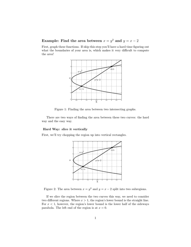
Example: Find the area between x = y 2 and y = x − 2
First, graph these functions. If skip this step you’ll have a hard time figuring out
what the boundaries of your area is, which makes it very difficult to compute
the area!
3
2
(4,2)
x=y2
Y
1
y=x−2
0
−1
(1,−1)
−2
−3
0
0.5
1
1.5
2
2.5
3
3.5
4
4.5
5
X
Figure 1: Finding the area between two intersecting graphs.
There are two ways of finding the area between these two curves: the hard
way and the easy way.
Hard Way: slice it vertically
First, we’ll try chopping the region up into vertical rectangles.
3
2
(4,2)
2
x=y
Y
1
y=x−2
0
−1
(1,−1)
−2
−3
0
0.5
1
1.5
2
2.5
3
3.5
4
4.5
5
X
Figure 2: The area between x = y 2 and y = x − 2 split into two subregions.
If we slice the region between the two curves this way, we need to consider
two different regions. Where x > 1, the region’s lower bound is the straight line.
For x < 1, however, the region’s lower bound is the lower half of the sideways
parabola. The left end of the region is at x = 0.
1
We must find the crossing points of the two curves; in other words, we find
the values of x and y that satisfy both equations simultaneously.
x = y2
and y = x − 2
so:
y−2
=
y2
y −y−2
=
0
(y − 2)(y + 1)
=
0
2
We conclude that:
y=2
or y = −1.
We can plug these values of y back in to either equation to find the associated
x values:
y = x−2
2 = x−2
4
=
x.
If we perform a similar equation with y = −1 we’ll find that the two points of
intersection are (1, −1) and (4, 2).
√
The equation of the upper
√ half of the sideways parabola is y = x and that
of the lower half is y = − x. The equation of the lower right hand boundary
of the region is just y = x − 2.
We find the area A between the two curves by integrating the difference
between the top curve and the bottom curve in each region:
top bottom-l
top
� 4 ���� bottom-r
����
� ��
� �� �
√ �
√
√
( x − (x − 2) ) dx
A=
( x − (− x) )) dx +
�0
��
� �1
��
�
left
right
�
1
The rest of this calculation is easy; just evaluate the integrals.
� 1
� 4
√
√
A = 2
x dx +
(−x + x + 2) dx
0
1
�1 �
�4
2
1
2
2 x3/2 + − x2 + x3/2 + 2x
3
2
3
�
�0 � 2
�1 �
�
2
4
2 3/2
1 2
−0 + − + ·4 +8 − − + +2
2
3
3
2
2 3
4
16
1 2
−8+
+8+ − −2
3
3
2 3
9
.
2
�
=
=
=
A
=
2
Easy Way: Slice it horizontally
There’s a much quicker way to complete this area calculation; you should look
for an easier way as soon as you notice the need to split the region into parts.
The quicker way is similar in principle but reverses the roles of x and y; in this
method we slice the area in question into horizontal rectangles.
3
2
x=y2
(4,2)
1
Y
dy
0
y=x−2
−1
(1,−1)
−2
−3
0
0.5
1
1.5
2
2.5
3
3.5
4
4.5
5
X
Figure 3: The area between x = y 2 and y = x − 2 and one horizontal rectangle.
The height of these rectangles is dy; we get their width by subtracting the
x-coordinate of the edge on the left curve from the x-coordinate of the edge on
the right curve. (If you get mixed up and subtract the right from the left you’ll
get a negative answer.) The left curve is the sideways parabola x = y 2 . The
right curve is the straight line y = x − 2 or x = y + 2.
The limits of integration come from the points of intersection we’ve already
calculated. In this case we’ll be adding the areas of rectangles going from the
bottom to the top (rather than left to right), so from y = −1 to y = 2.
�
A
y=2
=
�
�
(y + 2) − y 2 dy
y=−1
�2
−y 3
y2
+ 2y +
3
2 −1
�
� �
�
4
8
1
1
=
+4−
−
−2+
2
3
3
2
9
=
2
�
=
A
You’ll notice that if you plug the limits of integration into the integrand, you
get 0. This makes sense; as y goes toward −1 and 2 the width of the rectangles
approaches 0.
3
MIT OpenCourseWare
http://ocw.mit.edu
18.01SC Single Variable Calculus��
Fall 2010 ��
For information about citing these materials or our Terms of Use, visit: http://ocw.mit.edu/terms.