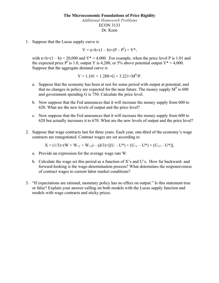
The Microeconomic Foundations of Price Rigidity
Additional Homework Problems
ECON 3133
Dr. Keen
1. Suppose that the Lucas supply curve is
Y = n×h×(1 – b)×(P – Pf) + Y*,
with n×h×(1 – b) = 20,000 and Y* = 4,000. For example, when the price level P is 1.01 and
the expected price Pf is 1.0, output Y is 4,200, or 5% above potential output Y* = 4,000.
Suppose that the aggregate demand curve is
Y = 1,101 + 1.288×G + 3.221×MS/P.
a. Suppose that the economy has been at rest for some period with output at potential, and
that no changes in policy are expected for the near future. The money supply MS is 600
and government spending G is 750. Calculate the price level.
b. Now suppose that the Fed announces that it will increase the money supply from 600 to
620. What are the new levels of output and the price level?
c. Now suppose that the Fed announces that it will increase the money supply from 600 to
620 but actually increases it to 670. What are the new levels of output and the price level?
2. Suppose that wage contracts last for three years. Each year, one-third of the economy’s wage
contracts are renegotiated. Contract wages are set according to
X = (1/3)×(W + W+1 + W+2) – (d/3)×[(U – U*) + (U+1 – U*) + (U+2 – U*)].
a. Provide an expression for the average wage rate W.
b. Calculate the wage set this period as a function of X’s and U’s. How far backward- and
forward-looking is the wage-determination process? What determines the responsiveness
of contract wages to current labor market conditions?
3. “If expectations are rational, monetary policy has no effect on output.” Is this statement true
or false? Explain your answer calling on both models with the Lucas supply function and
models with wage contracts and sticky prices.