ANALYSING LIKERT SCALE/TYPE DATA, ORDINAL LOGISTIC REGRESSION EXAMPLE IN R.
1. Motivation.
Likert items are used to measure respondents attitudes to a particular question or statement. One must recall
that Likert-type data is ordinal data, i.e. we can only say that one score is higher than another, not the distance
between the points.
Now lets imagine we are interested in analysing responses to some ascertion made, answered on a Liket scale as
below;
•
•
•
•
•
1
2
3
4
5
=
=
=
=
=
Strongly disagree
Disagree
Neutral
Agree
Strongly agree
2. Inference techniques.
Due to the ordinal nature of the data we cannot use parametric techniques to analyse Likert type data; Analysis
of variance techniques include;
• Mann Whitney test.
• Kruskal Wallis test.
Regression techniques include;
• Ordered logistic regression or;
• Multinomial logistic regression.
• Alternatively collapse the levels of the Dependent variable into two levels and run binary logistic regression.
2.1. Data. Our data consists of respondants answer to the question of interest, their sex (Male, Female), highest
post-school degree achieved (Bacheors, Masters, PhD, Other, None), and a standardised income related variable.
The score column contain the numerical equivalent scores to the respondants answers, and the nominal column
relats to a binning of respontants answers (where Neutral = 1, Strongly disagree or Disagree = 0, and Strongly agree
or Agree = 2). The first 6 respondants data are shown below;
> head(dat)
Answer sex
degree
income score nominal
1
Neutral
F
PhD -0.1459603
3
1
2
Disagree
F
Masters 0.8308092
2
1
3
Agree
F Bachelors 0.7433269
1
0
4 Stronly agree
F
Masters 1.2890023
5
2
5
Neutral
F
PhD -0.5763977
3
1
6
Disagree
F Bachelors -0.8089441
2
1
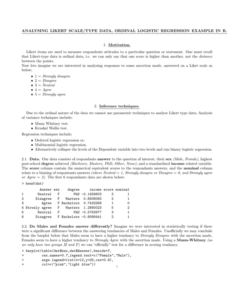
2.2. Do Males and Females answer differently? Imagine we were interested in statistically testing if there
were a significant difference between the answering tendancies of Males and Females. Unofficially we may conclude
from the barplot below that Males seem to have a higher tendancy to Strongly Disagree with the ascertion made,
Females seem to have a higher tendancy to Strongly Agree with the ascertion made. Using a Mann-Whitney (as
we only have two groups M and F) we can “officially” test for a difference in scoring tendancy.
> barplot(table(dat$sex,dat$Answer),beside=T,
+
cex.names=0.7,legend.text=c("Female","Male"),
+
args.legend=list(x=12,y=25,cex=0.8),
+
col=c("pink","light blue"))
1
ANALYSING LIKERT SCALE/TYPE DATA, ORDINAL LOGISTIC REGRESSION EXAMPLE IN R.
25
2
0
5
10
15
20
Female
Male
Agree
Disagree
Neutral
Strongly disagree
Stronly agree
2.2.1. Mann-Whitney test. To “officially” test for a difference in scoring tendancies between Males and Females we
use a Mann-Whitney (This is the same as a two-sample wilcoxon test).
> wilcox.test(score~sex,data=dat)
Wilcoxon rank sum test with continuity correction
data: score by sex
W = 3007, p-value = 0.04353
alternative hypothesis: true location shift is not equal to 0
From the Mann-Whitney test we get a p-value of 0.04353, hence we can reject the null hypothesis That Males and
Females have the same scoring tendancy at the 5% level. This is aslo evident from the bar chart which indicates
far more Females answer with Strongly Agree, and far more MAles answer with Strongly Disagree.
2.3. Do scoring tendancies differ by dregee level? If we were interested in statistically testing if there were
a significant difference between the scoring tendancies of people with different post-school degree cheivements.
Unofficially we may conclude from the barplot that there is seemilgly no difference in the scoring tendancies of
people having achieved either one of the listed degrees. Using a Kruskal-Wallis we can “officially” test for a
difference.
> barplot(table(dat$degree,dat$Answer),
+
beside=T,args.legend=list(cex=0.5),
+
cex.names=0.7,legend.text=c("Bachelors",
ANALYSING LIKERT SCALE/TYPE DATA, ORDINAL LOGISTIC REGRESSION EXAMPLE IN R.
"Masters","PhD","None","Other"))
12
+
>
3
0
2
4
6
8
10
Bachelors
Masters
PhD
None
Other
Agree
Disagree
Neutral
Strongly disagree
Stronly agree
2.3.1. Kruskal-Wallis Test. To “officially” test for a difference in scoring tendancies of people with different postschool degree cheivements we use a Kruskal-Wallis Test.
> kruskal.test(Answer~degree,data=dat)
Kruskal-Wallis rank sum test
data: Answer by degree
Kruskal-Wallis chi-squared = 7.5015, df = 4, p-value = 0.1116
The Kruskal-Wallis test gives us a p-vale of 0.1116, hence we have no evidence to reject our null hypothesis.
We are likely therefore to believe that there is no difference in scoring tendancy between people with different
post-school lvels of education.
2.3.2. One-Way ANOVA. One way of treating this type of data if we there is a “normally” distributed continious
independent variable is to flip the variables around. Hence, to ”officially” test for a difference in means between the
income of people scoring differently we use a One-way ANOVA (as the samples are independent).
> anova(lm(income~Answer,data=dat))
Analysis of Variance Table
Response: income
Df Sum Sq Mean Sq F value Pr(>F)
4
ANALYSING LIKERT SCALE/TYPE DATA, ORDINAL LOGISTIC REGRESSION EXAMPLE IN R.
Answer
4
6.699 1.67468 1.8435 0.1239
Residuals 139 126.273 0.90844
The ANOVA gives us a p-value of 0.1239, hece we have no evidence to reject our null-hypothesis. We are therefore
likely to believe that there is no difference in the average income of people who score in each of the five Likert
categories.
2.3.3. Chi-Square test. The Chi-Square test can be used if we combine the data into nominal categories, this
compares the observed numbers in each category with those expected (i.e. equal proportions), we asses if any
observed discrepancies (from our theory of equal proportions) can be reasonably put down to chance.
The numbers in each nominal category (as described above) are shown below;
> table(dat$nominal,dat$sex)
F M
0 16 14
1 40 45
2 28 1
> table(dat$nominal,dat$degree)
Bachelors Masters None Other PhD
0
6
5
11
5
3
1
7
5
27
30 16
2
3
11
7
4
4
>
Output from each Chi-square test is shown below. Initially we test if there is a significant difference between
the expected frequencies and the observed frequencies between the specified (nominal) scoring categories of the
sexes. The second Chi-squared test tests if there is a significant difference between the expected frequencies and
the observed frequencies between the specified (nominal) scoring categories of people with different post-school
education levels.
> chisq.test(table(dat$nominal,dat$sex))
Pearson's Chi-squared test
data: table(dat$nominal, dat$sex)
X-squared = 22.1815, df = 2, p-value = 1.525e-05
> chisq.test(table(dat$nominal,dat$degree))
Pearson's Chi-squared test
data: table(dat$nominal, dat$degree)
X-squared = 25.2794, df = 8, p-value = 0.001394
The first Chi-squared test gives us a p-value of < 0.001, hence we have a significant result at the 1% level allowing us
to reject the null hypothesis (of equal proportions). We would therefore believe that there are unequal proportions of
Males and Females scoring in each of the three (nominal) categories. The second Chi-squared test gives us a p-value
of < 0.002, hence we have a significant result at the 2% level allowing us to reject the null hypothesis (of equal
proportions). We would therefore believe that there are unequal proportions of people with different post-school
education levels scoring in each of the three (nominal) categories.
3. The Ordinal Logisic Regression Model.
Ordinal logistic regression or (ordinal regression) is used to predict an ordinal dependent variable given one or
more independent variables.
> library(MASS)
> mod<-polr(Answer~sex + degree + income, data=dat,Hess=T)
> summary(mod)
Call:
polr(formula = Answer ~ sex + degree + income, data = dat, Hess = T)
Coefficients:
ANALYSING LIKERT SCALE/TYPE DATA, ORDINAL LOGISTIC REGRESSION EXAMPLE IN R.
5
Value Std. Error t value
sexM
-1.1084
0.4518 -2.453
degreeMasters 1.8911
0.6666
2.837
degreeNone
1.5455
0.6398
2.415
degreeOther
1.9284
0.6511
2.962
degreePhD
1.0565
0.5883
1.796
income
-0.1626
0.1577 -1.031
Intercepts:
Value
Std. Error t value
Agree|Disagree
-0.4930 0.4672
-1.0553
Disagree|Neutral
0.7670 0.4754
1.6134
Neutral|Strongly disagree
1.7947 0.4951
3.6245
Strongly disagree|Stronly agree 2.4345 0.5113
4.7617
Residual Deviance: 437.2247
AIC: 457.2247
The summary output in R gives us the estimated log-odds Coefficients of each of the predictor varibales shown
in the Coefficients section of the output. The cut-points for the adjecent levels of the response variable shown in
the Intercepts section of the output.
Standard interpretation of the ordered log-odds coefficient is that for a one unit increase in the predictor, the
response variable level is expected to change by its respective regression coefficient in the ordered log-odds scale
while the other variables in the model are held constant. In our model Female and Bachelors are included in the
baseline for the model as both sex and degree are factor variables, so for a Male with a Masters degree his ordered
log-odds of scoring in a higher category would increase by −1.1084 + 1.8911 = 0.77827 over the factors included in
the baseline.
Interpreting the estimate of the coefficient for the “income” variable tells us that for one unit incerease in the income
variable the ordered log-odds of scoring in a higher category decreases by 0.1626 with the other factors in the model
being held constant.
The cutpoints are used to differentiate the adjacent levels of the response variable, i.e.( points on a continuous
unobservable phenomena, that result in the different observed values on the levels of the dependent variable used to
measure the unobservable variable). Hence Agree|Disagree, is used do differentiate the other levels of the response
variable when the values of the predictor variables are set to zero. Interpretation of this may be that people who
had a value of -0.4930 or less on the underlying unobserved variable that gave rise to the Answer would be classified
as lower scoring given that they were Female with a Bachelors (the baseline variables) and had all othe variables
set to zero.
R doesn’t calculate the associated p-values for each coefficient by deafault, hence below is the R code to do this (to
3 decimal places);
> coeffs <- coef(summary(mod))
> p <- pnorm(abs(coeffs[, "t value"]), lower.tail = FALSE) * 2
> cbind(coeffs, "p value" = round(p,3))
Value Std. Error
t value p value
sexM
-1.1083975 0.4518069 -2.453255
0.014
degreeMasters
1.8911478 0.6665792 2.837094
0.005
degreeNone
1.5454807 0.6398273 2.415465
0.016
degreeOther
1.9283955 0.6511113 2.961698
0.003
degreePhD
1.0564763 0.5882532 1.795955
0.073
income
-0.1626251 0.1577345 -1.031005
0.303
Agree|Disagree
-0.4929701 0.4671580 -1.055253
0.291
Disagree|Neutral
0.7670239 0.4753955 1.613444
0.107
Neutral|Strongly disagree
1.7946651 0.4951443 3.624530
0.000
Strongly disagree|Stronly agree 2.4345280 0.5112730 4.761699
0.000
Above are the test statistics and p-values, respectively for the null hypothesis that an individual predictor’s regression coefficient is zero given that the rest of the predictors are in the model. We note that we can reject this
null hypothesis for the predictors degreeOther and degreeMasters with associated p-values 0.005 and 0.003
6
ANALYSING LIKERT SCALE/TYPE DATA, ORDINAL LOGISTIC REGRESSION EXAMPLE IN R.
respectively. Interpretation for these p-values is similar to any other regression analysis.
The Odds ratios are simply the inverse log (i.e. the exponential) of the estimated coefficients, code for doing this
in R is shown below;
> exp(coef(mod))
sexM degreeMasters
0.3300875
6.6269710
income
0.8499098
degreeNone
4.6902255
degreeOther
6.8784647
degreePhD
2.8762181
Interpreting these Odds ratios we are essentially comparing the people who are in groups greater than x versus
those who are in groups less than or equal to x, where x is the level of the response variable. Hence for a one unit
change in the predictor variable, the odds for cases in a group that is greater than x versus less than or equal to
x are the proportional odds times larger. So for say the “income” variable a one unit increase in this variable, the
odds of high “Answer” versus the combined adjacent “Answer” categories are 0.8499098 times greater, given the
other variables are held constant in the model.
4. Analysing Likert scale data.
A Likert scale is composed of a series of four or more Likert-type items that represent similar questions combined
into a single composite score/variable. Likert scale data can be analyzed as interval data, i.e. the mean is the best
measure of central tendency.
4.1. Inference.. Parametric analysis of ordinary averages of Likert scale data is justifiable by the Central Limit
Theorem, analysis of variance techniques incude;
• t-test.
• ANOVA.
• Linear regression procedures
4.2. Motivation. If we consider the situation where we had five such questions each scored on the same Likert
type items (on a numerical scale), we would simply sum each respondants answer to create a single score. The first
few rows of the data analysed can be seen below;
> head(dataframe)
qu1
qu2
qu3
qu4
qu5 sex
1
Neutral Stronly agree
Disagree
Neutral
Neutral
F
2
Disagree
Neutral Stronly agree Stronly agree Stronly agree
F
3
Agree
Agree Stronly agree
Agree
Disagree
F
4 Stronly agree Stronly agree Stronly agree
Agree Stronly agree
F
5
Neutral
Disagree
Neutral
Disagree
Neutral
F
6
Disagree
Neutral
Disagree
Neutral
Agree
F
degree
income sum
1
PhD -0.1459603 16
2
Masters 0.8308092 20
3 Bachelors 0.7433269 10
4
Masters 1.2890023 21
5
PhD -0.5763977 13
6 Bachelors -0.8089441 11
>
Where qu1, qu2,qu3,au4, and qu5 are the columns containing the respondants answers to the 5 questions, sex,
degree and income are the same as above. The sum column contains the sums of each respondants answers to
questions 1 to 5.
4.3. Parametric Inference.
ANALYSING LIKERT SCALE/TYPE DATA, ORDINAL LOGISTIC REGRESSION EXAMPLE IN R.
7
4.3.1. Normality.
20
15
0
5
10
Frequency
25
30
> hist(dataframe$sum,xlab="Sum of scores",main="")
10
15
20
Sum of scores
From the histogram above we can “unofficially” conclude that our data is relitively Normal, hance we are somewhat
justified in using parametric statistical methodology.
4.3.2. T-Test. We can use a two-sample T-test to asses if there is a difference in the average scores of Males and
Females.
> boxplot(sum~sex,data=dataframe,names=c("Female","Male"),
+
ylab="Sum of scores")
ANALYSING LIKERT SCALE/TYPE DATA, ORDINAL LOGISTIC REGRESSION EXAMPLE IN R.
15
10
Sum of scores
20
8
Female
Male
> t.test(sum~sex,data=dataframe)
Welch Two Sample t-test
data: sum by sex
t = 1.9879, df = 136.6, p-value = 0.04882
alternative hypothesis: true difference in means is not equal to 0
95 percent confidence interval:
0.005887951 2.246493001
sample estimates:
mean in group F mean in group M
14.22619
13.10000
The t-test gives us a p-value of 0.04882 which is significant at the 5% level, hence we have evidence to reject the
null hypothesis. We are therefore likely to believe that the avarage scores of Males and Females are unequal, from
the boxplot and the mean estimates given in the R output we can conclude that on average Males score lower than
Females.
4.3.3. Two-way ANOVA.. The Two-way ANOVA is used to simultaneously asses if there is a difference between
the average scores of people of different sex, post-school education level and income score.
> boxplot(sum~degree,data=dataframe,
+
names=c("Bachelors","Masters","PhD","None","Other"),
+
ylab="Sum of scores")
>
9
15
10
Sum of scores
20
ANALYSING LIKERT SCALE/TYPE DATA, ORDINAL LOGISTIC REGRESSION EXAMPLE IN R.
Bachelors
Masters
PhD
None
Other
> anova(lm(sum~sex+degree+income,data=dataframe))
Analysis of Variance Table
Response: sum
Df Sum Sq Mean Sq F value Pr(>F)
sex
1
44.39 44.391 3.9817 0.04798 *
degree
4 138.09 34.522 3.0965 0.01778 *
income
1
6.64
6.645 0.5960 0.44142
Residuals 137 1527.37 11.149
--Signif. codes: 0 '***' 0.001 '**' 0.01 '*' 0.05 '.' 0.1 ' ' 1
The two-way ANOVA output indicates a significant diference of average scores between sexes (a p-value of 0.04798)
and peple with different post-scool level of education (a p-value of 0.01778), but no significant difference relating
to average “income” (accounting for the inclusion of the other variables in the model). From the boxplot we may
unofficially conclude that the significant difference in post-school education arises from the scoring of Masters
graduates, however further post-hoc analysis would be required to “officially” conclude where the differences lie.
The t-test carried out above allows us to see where the significance difference between sexes arises from.