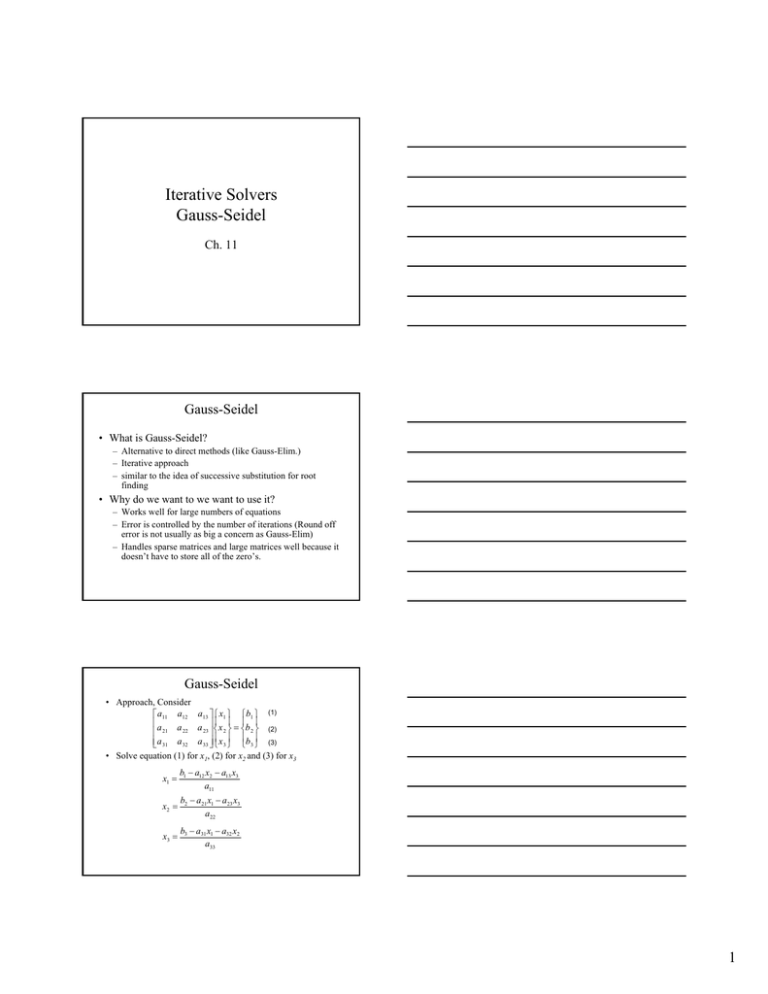
Iterative Solvers
Gauss-Seidel
Ch. 11
Gauss-Seidel
• What is Gauss-Seidel?
– Alternative to direct methods (like Gauss-Elim.)
– Iterative approach
– similar to the idea of successive substitution for root
finding
• Why do we want to we want to use it?
– Works well for large numbers of equations
– Error is controlled by the number of iterations (Round off
error is not usually as big a concern as Gauss-Elim)
– Handles sparse matrices and large matrices well because it
doesn’t have to store all of the zero’s.
Gauss-Seidel
• Approach, Consider
⎡ a11 a12 a13 ⎤ ⎧ x1 ⎫ ⎧ b1 ⎫ (1)
⎢a
⎥⎪ ⎪ ⎪ ⎪
⎢ 21 a 22 a 23 ⎥ ⎨ x 2 ⎬ = ⎨b 2 ⎬ (2)
⎢⎣a 31 a 32 a 33 ⎦⎥ ⎪⎩ x 3 ⎪⎭ ⎪⎩b 3 ⎪⎭ (3)
• Solve equation (1) for x1, (2) for x2 and (3) for x3
x1 =
b1 − a12 x2 − a13 x3
a11
x2 =
b2 − a21 x1 − a23 x3
a22
x3 =
b3 − a31 x1 − a32 x2
a33
1
Gauss-Seidel - Method
• Start iteration process by guessing x02 and x03 and always
using the most recent values of x’s
b −a x −a x
x1 = 1 12 2 13 3
x11 → x20 , x20
a11
x12 → x11 , x30
b2 − a21 x1 − a23 x3
x2 =
a22
x31 → x11 , x12
b −a x −a x
x3 = 3 31 1 32 2
Repeat using the new x’s
a33
• Check for convergence:
ε a ,i =
x ik − x ik −1
x ik
×100%
For all i’s where k = current iteration, k-1 = previous iterations
Gauss-Seidel – Convergence criteria
• Diagonal Dominance – the diagonal element of a row
should be greater than the sum of all other row elements
n
aii > ∑ aij
j =1
j ≠i
⎡1 3 5 ⎤
⎢2 5 7 ⎥
⎢
⎥
⎢⎣3 1 1 ⎥⎦
Is this matrix
diagonally dominant?
• Sufficient but not necessary (I.e., if the condition is
satisfied, convergence is guaranteed, if the condition is
NOT satisfied, convergence still may occur
Gauss-Seidel – Relaxation for iterative methods
• Motivation – speed up convergence – assuming we know
the direction of the solution
x
k +1
extrapolated solution
*
New solution
k
iterations (k)
1
λ
• Linear Extrapolation
x* − x k x k +1 − x k
=
1
λ
x k +1 = x k + λ (x * − x k )
x k +1 = λx* + (1 − λ )x k
2
Gauss-Seidel – Relaxation for iterative methods
• Motivation – speed up convergence – assuming we know
the direction of the solution
x
k +1
extrapolated solution
*
New solution (present value)
k
iterations (k)
1
λ
• Linear Extrapolation
x* − x k x k +1 − x k
=
1
λ
k +1
k
x = x + λ (x * − x k )
λ relaxation coefficient
x k +1 = λx* + (1 − λ )x k
Gauss-Seidel – Relaxation for iterative methods
What is x* ?
•
x1* =
b1 − a12 x2k − a13 x3k
a11
Relaxation Coefficient – λ
•
–
Typical Values: 0 < λ < 2
1.
2.
–
–
–
3.
x k +1 = λx* + (1 − λ )x k
No relaxation : λ = 1
Underrelaxation: 0 < λ < 1
Provides a weighted average of current & previous results
Used to make non-convergent systems converge
Helps speed up convergence by damping oscillations
Overrelaxation: 1 < λ < 2
–
–
–
–
Extra emphasis placed on present value
Assumes the solution is preceeding to the desired result, just too slowly
Will speed up convergence of a system that is already convergent
Selection of λ is problem specific and can require trial and error
Gauss-Seidel – Pseudocode
1st Loop: Row Normalization (divide all terms in the
equation by diagonal term)
2nd Loop: Rearrange Equations:
x1 = b1 − a12 x2 − a13 x3 − ⋅ ⋅ ⋅
•
•
–
•
Note a11 = 1 after normalization
Error checking flag – set to 1 at the beginning of each
loop
–
–
Change to zero if any εa > εs
No need to check any εa’s after that – saves computations
Show Matlab Gauss-Seidel Example
3
Other Iterative Solvers and GS varients
•
Jacobi method – GS always uses the newest value of the
variable x, Jacobi uses old values throughout the entire
iteration
•
Iterative Solvers are regularly used to solve Poisson’s
equation in 2 and 3D using finite
difference/element/volume discretizations:
∂ 2T ∂ 2T ∂ 2T
+
+
= f ( x, y , z )
∂x 2 ∂y 2 ∂z 2
•
Red Black Gauss Seidel
•
Multigrid Methods
•
Determine the force in each member of the truss and the
reaction forces
Engineering Application
400
45ο
45ο
200
60ο
30ο
4