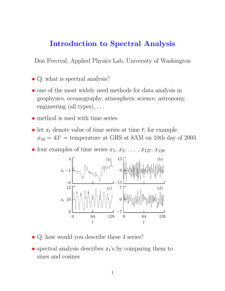
Introduction to Spectral Analysis
Don Percival, Applied Physics Lab, University of Washington
• Q: what is spectral analysis?
• one of the most widely used methods for data analysis in
geophysics, oceanography, atmospheric science, astronomy,
engineering (all types), . . .
• method is used with time series
• let xt denote value of time series at time t; for example,
x10 = 43◦ = temperature at GHS at 8AM on 10th day of 2003
• four examples of time series x1, x2, . . . , x127, x128
4
(a)
15
xt −1
0
−6
12
−15
7
(c)
xt 10
0
8
0
64
t
128
−7
(b)
(d)
0
64
t
128
• Q: how would you describe these 4 series?
• spectral analysis describes xt’s by comparing them to
sines and cosines
1
Sines and Cosines: I
• Q: what do sines and cosines have to do with time series?
• plots of sin(u) and cos(u) versus u as u goes from 0 to 4π
2
0
−2
0
2π
u
4π 0
2π
u
4π
2
• let u = 2π 128
t for t = 1, 2, . . . , 128
2
2
t) and cos(2π 128
t) versus t
• plots of sin(2π 128
2
0
−2
0
64
t
128 0
64
t
128
2
• can regard above as artificial time series: st = sin(2π 128
t) etc
• can interpret
2
128
as ‘2 cycles over time span of 128’
2
Sines and Cosines: II
7
• now let u = 2π 128
t for t = 1, 2, . . . , 128
7
7
t) and cos(2π 128
t) versus t
• plots of sin(2π 128
2
0
−2
0
64
t
128 0
64
t
128
• now get series with 7 cycles over time span of 128
k
t) etc versus t have k cycles
• in general plots of sin(2π 128
k
is called frequency of sine or cosine
• quantity 128
(usually use variable f to denote frequency)
if k is small, sine time series is said to have low frequency
if k is large, sine time series is said to have high frequency
k
• amplitude (maximum range of variation) of st = sin(2π 128
t) is 1
7
7
t) and 1.5 sin(2π 128
t)
• plots of 0.5 sin(2π 128
2
0
−2
0
64
t
128 0
3
64
t
128
Sines and Cosines: III
• let’s add together sines and cosines with different frequencies
first column uses sines and cosines of amplitude 1
second and third columns use random amplitudes
f=
1
128
f=
3
128
f=
5
128
f=
7
128
f=
9
128
f=
11
128
f=
13
128
f=
15
128
f=
17
128
f=
19
128
xt
0
128 0
t
128 0
t
128
t
• conclusion: by summing up lots of sines and cosines with different
amplitudes, can get artificial time series that resemble actual
time series
4
Goal of Spectral Analysis
• given a time series xt, figure out how to construct it using sines
and cosines; i.e., to write
k
k
xt =
ak sin(2π 128
t) + bk cos(2π 128
t)
k
• above called ‘Fourier representation’ for a time series
(named after 19th Century French mathematician)
• allows us to reexpress time series in a standard way
• different time series will need different ak ’s and bk ’s
• can compare different time series by comparing the ak ’s and bk ’s
5
Gory Details: I
• Q: how do we figure out what ak ’s and bk ’s should be to form a
particular time series?
• answer turns out to be surprisingly simple:
1 1 k
k
ak =
xt sin(2π 128 t) and bk =
xt cos(2π 128
t)
64 t=1
64 t=1
128
128
• to see why this is reasonable, consider the following:
let y1, . . . , y128 & z1, . . . , z128 be collections of ordered values
1
let ȳ and z̄ be their sample means (i.e., ȳ = 128
t yt etc.)
let σy2 and σz2 be their sample variances: i.e.,
σy2 =
1
128
128
(yt − ȳ)2
t=1
sample correlation coefficient:
1
(y
−
ȳ)(z
−
z̄)
t
t
t yt zt
ρ̂ = 128 t
=
,
σy σz
128σy σz
where 2nd equality holds if z̄ = 0
measures strength of linear relationship between yt’s and zt’s
(−1 ≤ ρ̂ ≤ 1)
relationship is strong if t ytzt is large in magnitude
ak is thus related to strength of linear relationship between
k
yt = xt and zt = sin(2π 128
t), for which z̄ = 0
6
Gory Details: II
k
• to summarize how important frequency 128
is in
k
k
ak sin(2π 128
t) + bk cos(2π 128
t),
xt =
k
let us form Sk = 12 (a2k + b2k )
if frequency
if frequency
k
128
k
128
is important, then Sk should be large
is not important, then Sk should be small
• Sk over all frequencies
k
128
is called the spectrum
• fundamental fact about the spectrum:
k
Sk =
1
128
128
(xt − x̄)2 = σx2
t=1
i.e., spectrum breaks sample variance of time series up into pieces,
each of which is associated with a particular frequency
• spectral analysis is thus an analysis of variance technique,
in which σx2 is broken up across different frequencies
7
Examples of Spectral Analysis
• recall the four examples of time series
4
15
(a)
xt −1
0
−6
12
−15
7
(c)
xt 10
0
8
0
64
t
128
−7
(b)
(d)
0
64
t
128
• here are the spectra for these four series
(a)
(b)
(c)
(d)
Sk
Sk
0
0.25
k
f = 128
0.5 0
0.25
k
f = 128
0.5
• uses include testing theories (e.g., wind data), exploratory data
analysis (e.g., rainfall data), discriminating data (e.g., neonates),
assessing predictability (e.g., atomic clocks)
8