Dr. W. Pezzaglia
LPC Physics
Physics 2A Lab, Fall 2012
Lab #1 Galileo’s Law
Page 1
2012Aug21
Lab 1: Galileo’s Law of Inclined Planes
Preparation for Lab
 Read Knight chapter 2 on constant accelerated motion (inclined planes)
 Virtual Museum (2 min): http://catalogue.museogalileo.it/multimedia/InclinedPlane.html
 Video Introduction Nova (4 min):
http://www.teachersdomain.org/resource/phy03.sci.phys.mfw.galileoplane/
 Video Introduction: Mechanical Universe #2, Law of Falling Bodies (30 min):
http://video.google.com/videoplay?docid=3641917188010584794#
==================================================================
Theory:
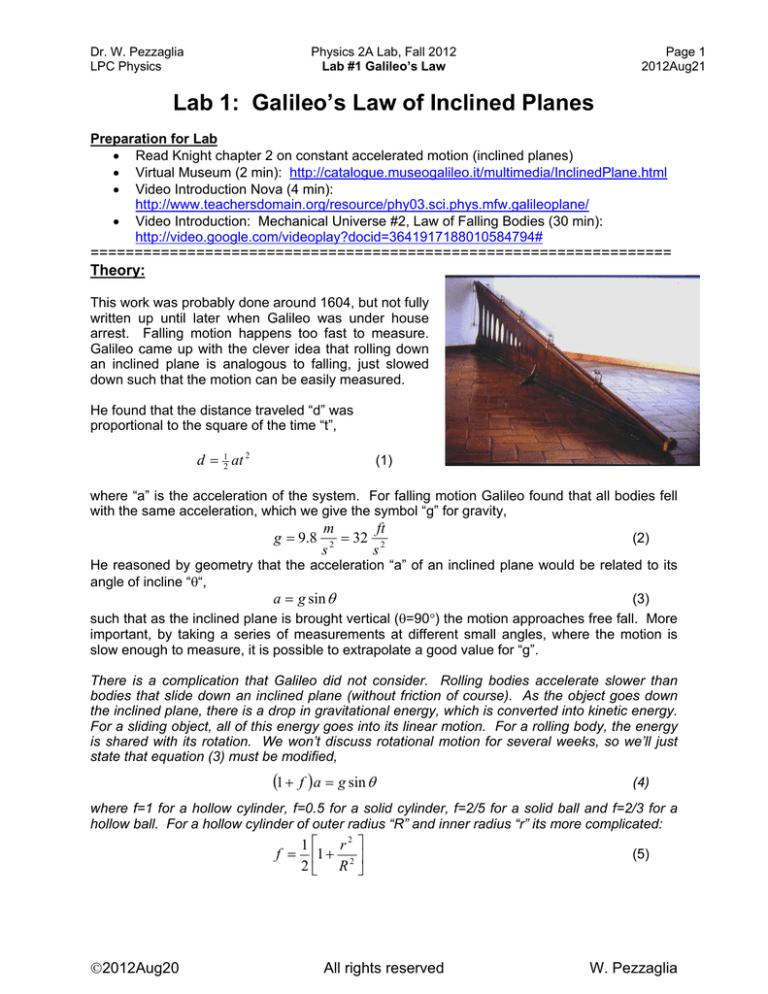
This work was probably done around 1604, but not fully
written up until later when Galileo was under house
arrest. Falling motion happens too fast to measure.
Galileo came up with the clever idea that rolling down
an inclined plane is analogous to falling, just slowed
down such that the motion can be easily measured.
He found that the distance traveled “d” was
proportional to the square of the time “t”,
d  12 at 2
(1)
where “a” is the acceleration of the system. For falling motion Galileo found that all bodies fell
with the same acceleration, which we give the symbol “g” for gravity,
g  9.8
m
ft
 32 2
2
s
s
(2)
He reasoned by geometry that the acceleration “a” of an inclined plane would be related to its
angle of incline ““,
a  g sin 
(3)
such that as the inclined plane is brought vertical (=90) the motion approaches free fall. More
important, by taking a series of measurements at different small angles, where the motion is
slow enough to measure, it is possible to extrapolate a good value for “g”.
There is a complication that Galileo did not consider. Rolling bodies accelerate slower than
bodies that slide down an inclined plane (without friction of course). As the object goes down
the inclined plane, there is a drop in gravitational energy, which is converted into kinetic energy.
For a sliding object, all of this energy goes into its linear motion. For a rolling body, the energy
is shared with its rotation. We won’t discuss rotational motion for several weeks, so we’ll just
state that equation (3) must be modified,
1  f  a  g sin 
(4)
where f=1 for a hollow cylinder, f=0.5 for a solid cylinder, f=2/5 for a solid ball and f=2/3 for a
hollow ball. For a hollow cylinder of outer radius “R” and inner radius “r” its more complicated:
1  r2 
f  1  2 
2 R 
2012Aug20
All rights reserved
(5)
W. Pezzaglia
Dr. W. Pezzaglia
LPC Physics
Physics 2A Lab, Fall 2012
Lab #1 Galileo’s Law
Page 2
2012Aug21
Experiment:
Part A: Setup

Measure total length of inclined plane “L” (if it’s a board its just the length of the board. If
you are using the whole table, then it’s the distance between the legs of the table).

Measure the amount “h” that you have lifted one end of the board (table). [For a 1 meter
length board, suggest that h  3 cm else it will go too fast, for 2 meters, keep h  6 cm].

Sketch your setup in your lab book with the dimensions labeled.
Question 1 Phenomena Test 1: Size of ball
a) Prediction: If we roll two different sized balls down the inclined plane at the same time,
which should get to the bottom first? Why?
b) Experiment: do the experiment!
c) Observation: What do you observe?
d) Analyze: Summarize what you have learned!
Question 2 Phenomena Test 2: Shape of object
a) Prediction: If we roll a ball and a cylinder down the inclined plane at the same time, which
should get to the bottom first? Why?
b) Do the experiment!
c) What do you observe?
d) Summarize
Question 3 Object Information for rest of experiments
a) Select one of your objects to use for the rest of experiment. Which one is it? (Hollow
cylinder, disk, ball etc).
b) Sketch the object and show its dimensions
c) What is its mass (if known or you can measure it)*?
d) What is the (fudge) factor “f” for your object?
Question 4 Inclined Plane: Theoretical Calculation
a) What is the length “L” of the plane (hypotenuse)?
b) By how much “h” have you lifted one end (leg) of the board (table)?
c) What then is the angle of incline? [Hint:
h
 sin  ]
L
d) From equation (4) what then is the expected acceleration “a” for rolling motion?
=================================================================
*Note, if you are using one of the BIG rings, you probably can’t measure the mass with our
small scales.
2012Aug20
All rights reserved
W. Pezzaglia
Dr. W. Pezzaglia
LPC Physics
Physics 2A Lab, Fall 2012
Lab #1 Galileo’s Law
Page 3
2012Aug21
Part B: Distance vs Time

Measure travel time as a function of distance, holding slope unchanged.

If plane is 1 meters long, suggest use distances d= 100, 70, 50 and 25 cm. [If your board is
closer to 2 meters, then 200 cm, 150 cm, 100 cm, 50 cm]. Note that you sometimes have to
start 2 or 3 cm from edge of board to get it to roll.

Repeat each time measurement 4 times, take average.

Use supplied Excel Template: Type in your data, it will
a) take averages for you
b) Plot distance vs squared time
c) Fit plot with best line, determine slope
d) from slope calculate acceleration: a  2  Slope
Question 5 Analysis of Plot
a) Does your plot validate equation (1)? [In other words, does the plot show a line, which tells
us that distance is proportional to squared time]
b) What is the “R squared” value of the linear fit? Is it close to 1 (i.e. a “good” fit)?
c) What is the slope of the linear fit? [be sure to have correct units]
d) What is the (absolute) uncertainty in the slope? The percent uncertainty?
Question 6 Compare to known value
a) From the slope, determine the measured acceleration of the system. [ a  2  Slope ]
b) Compare to the theoretical value in question 4d. Compare means you calculate the “error”
 absolute error=measured – true value
 percent error = 100%(absolute error)/(true value)]
c) Is your error smaller than the (percent) uncertainty in the slope?
d) Is your percent error smaller than 5%?
Notes: Dr. Bill usually gets results to agree to within 2% or better.
=================================================================
2012Aug20
All rights reserved
W. Pezzaglia
Dr. W. Pezzaglia
LPC Physics
Physics 2A Lab, Fall 2012
Lab #1 Galileo’s Law
Page 4
2012Aug21
Sample Analysis for Part B
Group #
1
Run
1
2
3
4
Slope
STEYX
STDEV
num pts
Unc slope
Unc slope
Names
Dr. Bill
Date
6/26/2012
h (cm) Degrees d (cm) T1 (sec) T2 (sec) T3 (sec) T4 (sec) T avg T2
1.0
0.29
200
12.1
13.2
12.5
12.8 12.65
160.0
1.0
0.29
150
10
9.9
11.4
11.9 10.80
116.6
1.0
0.29
100
9.1
9.4
9
9.3 9.20
84.6
1.0
0.29
50
6
6.1
6.6
5.8 6.13
37.5
m
y
x
N
m

1.25
5.49
51.7
4
0.05
4.3%
cm/s2
cm
s2
points
cm/s2
Brd Len
L
Theory Ffactor
Theory Accel
Meas
Accel
Error
200 cm
1.0
2.48 cm/s2
2.49 cm/s2
0.4%
Hollow cylinder down Inclined Plane (0.29 degrees)
250
y = 1.2455x + 0.8209
R² = 0.9952
Distance (cm)
200
150
100
50
0
0.0
50.0
100.0
150.0
200.0
Squared Time (seconds)
2012Aug20
All rights reserved
W. Pezzaglia
Dr. W. Pezzaglia
LPC Physics
Physics 2A Lab, Fall 2012
Lab #1 Galileo’s Law
Page 5
2012Aug21
Part C: Acceleration vs angle of incline

Measure travel time as a function of height “h” of incline. Try to keep distance “d” constant.

Suggest use approximately h=1.5 cm and 3 cm if length is 100 cm (double it if 200 cm)

Repeat each time measurement 4 times, take average of times.

Repeat measurements with plane tilted in other direction (this cancels out leveling errors).
Note these heights will be “negative” to represent going other way.

Use Excel Template: it will
a) Calculate average times
b) Calculate the acceleration for the average time: a 
2d
t2
c) Plot acceleration “a” vs height “h”. [For backwards tilts, let both “a” and “h” be called
negative.]
d) Fit best line (get Rsquared, slope “m” and intercept).

From slope “m” you can get the acceleration of gravity: g  mL(1  f )
Question 7 Summary of the Plot
a) Is the plot a line as expected? (R squared value?)
b) Discuss how this validates the form of equation (4).
c) What is the slope? (be sure to have correct units)
d) What is the uncertainty in the slope?
Question 8 Analysis
a) From the slope, what is your measured acceleration of gravity? [ g  mL(1  f ) ]
b) The percent uncertainty in this quantity is the same as percent uncertainty in slope.
c) Compare your measured value to the known value for “g”. [What is your percent error?]
d) Is your error smaller than the uncertainty?
Question 9 Leveling Error
a) What is the intercept of your plot? Is it zero?
b) A non zero intercept tells you that “h” has a leveling error. By what angle is your table not
level?
c) Check the leveling of table with a bubble level. Does it show the table is unleveled?
Notes: Dr. Bill usually gets results to agree to within 2% or better.
=================================================================
2012Aug20
All rights reserved
W. Pezzaglia
Dr. W. Pezzaglia
LPC Physics
Physics 2A Lab, Fall 2012
Lab #1 Galileo’s Law
Page 6
2012Aug21
Example: Part C: Analysis Fixed Length, Change angle of incline
h (cm) Degrees d (cm) T1 (sec) T2 (sec) T3 (sec) T4 (sec) T avg a cm/s2
1.0
2.25
0.3
200
13.2
13.4
12.9
13.8 13.33
2.0
4.32
0.6
200
9.7
9.6
9.5
9.7 9.63
-1.0
-2.19
-0.3
200
13.8
13.3
13.1
13.9 13.53
-3.0
-6.75
-0.9
200
7.7
7.7
7.9
7.5 7.70
Run
1
2
3
4
Slope
STEYX
STDEV
num pts
Unc slope
Unc slope
m
y
x
N
m

2.22
0.10
2.2
4
0.02
1.0%
cm/s2
cm
s2
points
cm/s2
Leg Dist
L
Theory Ffactor
Theory g
Meas
g
Error
225 cm
1.0
980.00 cm/s2
998.36 cm/s2
1.9%
Hollow Cylinder rolling down different Inclined Planes
6.00
y = 2.2186x - 0.036
R2 = 0.9997
4.00
Acceleration (cm/s2)
2.00
0.00
-4.0
-3.0
-2.0
-1.0
0.0
1.0
2.0
3.0
-2.00
-4.00
-6.00
-8.00
Spacer Height (cm)
2012Aug20
All rights reserved
W. Pezzaglia
Dr. W. Pezzaglia
LPC Physics
Physics 2A Lab, Fall 2012
Lab #1 Galileo’s Law
Page 7
2012Aug21
Supplementary Notes on using Excel and Uncertainties
To get slope and intercept in Excel:
Slope Function:
m=SLOPE(y values, x values)
Intercept Function
b=INTERCEPT(y values, x values)
R Squared Test Value
R2=RSQ(y values, x values)
m 
Uncertainty in Slope:
y
x N
Where N= number of points
Where Standard Error in Y values:
y  STEYX(y values, x values)
Where Standard Deviation of X values:
x STDEV(x values)
b 
Uncertainty in Intercept:
y
N

1   x
 x



2
Where N= number of points
Where Standard Error in Y values:
y  STEYX(y values, x values)
Where Standard Deviation of X values:
x STDEV(x values)
Where Average of X values:
x=AVERAGE(x values)
Propagation of Uncertainties:
Recall absolute uncertainty in addition or subtraction is a sum in quadrature of the absolute
uncertainties.

Example, if z=xy, then  z   x   y
2
2
Recall percent uncertainty in multiplication or division is a sum in quadrature of the percent
uncertainties.

   y
  x   
Example, if z=xy, or z=x/y, then
z
 x   y
z
2



2
Recall percent uncertainty in a N-th power, is N times the percent uncertainty.

Example, if z  x N , then
 
 N x 
z
 x 
z
Misc:

Absolute Error=(Measured Value)-(True Value)

Percent Error=100%(Absolute Error)/(True Value)=100%[(Measured)/(True)-1 ]
2012Aug20
All rights reserved
W. Pezzaglia